
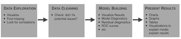
Exploratory Data Analysis, or EDA, is essentially a type of storytelling for statisticians. It allows us to uncover patterns and insights, often with visual methods, within data. EDA is often the first step of the data modelling process. In this phase, data engineers have some questions in hand and try to validate those questions by performing EDA.
EDA may sound exotic if you are new to the world of statistics. However, it’s not actually very difficult to perform an EDA. Nor do you need to know special languages to do it. As this article shows, you can use Python to do an EDA at any point in the Machine Learning (ML) process:
All the code, processes and data you need to follow along can be found in my EDA Gitub repo.
Installing Python and Pandas
If you already have Python installed, you can skip this step. However for those who haven’t, read on!
For this tutorial, I will be using ActiveState’s Python. There’s no major difference between the open source version of Python and ActiveState’s Python – for a developer. However, ActiveState Python is built from vetted source code and is regularly maintained for security clearance.
For this tutorial, you have two choices:
1. Download and install the pre-built “Exploratory Data Analysis” runtime environment for CentOS 7, or
2. If you’re on a different OS, you can automatically build your own custom Python runtime with just the packages you’ll need for this project by creating a free ActiveState Platform account, after which you will see the following image:

3. If you click the Get Started button you can choose Python, the OS you are working in, and then add “pandas,” “seaborn,” and “matplotlib” from the list of packages available.
4. Once the runtime builds, you can you can download the State Tool and use it to install your runtime:
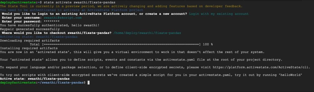
And that’s it! You now have Python installed with all the required packages. If you want to read a more detailed guide on how to install ActivePython on Linux, please read here.
In this directory, create your first “eda.py” file.
Choosing a Dataset
For the purpose of this tutorial, we will be using a CSV file containing the sale prices of houses and their attributes. You can find it on the previously mentioned Github repository here.
A quick look at the dataset using “df.columns” shows:
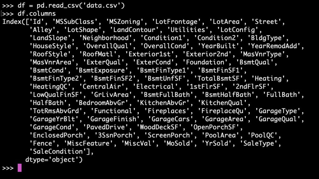
You can explore the dataset further by looking at the number of features, number of rows, the datatype of each column, and so on.
Exploring a Dataset
A quick look at the dataset can be done by calling on the Pandas “info” method, like so:
This shows us the number of non-null cells for each column. It is obvious from this data that the columns, MiscFeature (55), Fence (281), PoolQC (7), and Alley (91) are not relevant to building a model as they are present in far fewer quantities.
All these columns can be dropped.
Distributions
The data describes house sale prices against house attributes. In order for the data model to learn accurately, we need to train it with data that does not have too many outliers. Testing data should ideally be a narrow representation of a single problem.
To visualize the distribution of the sale price:
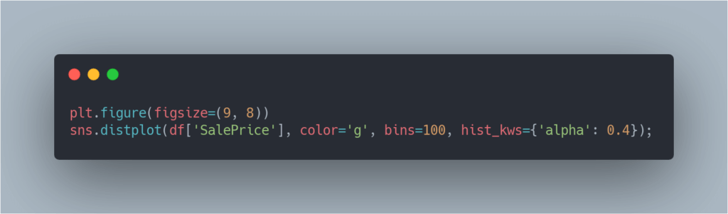
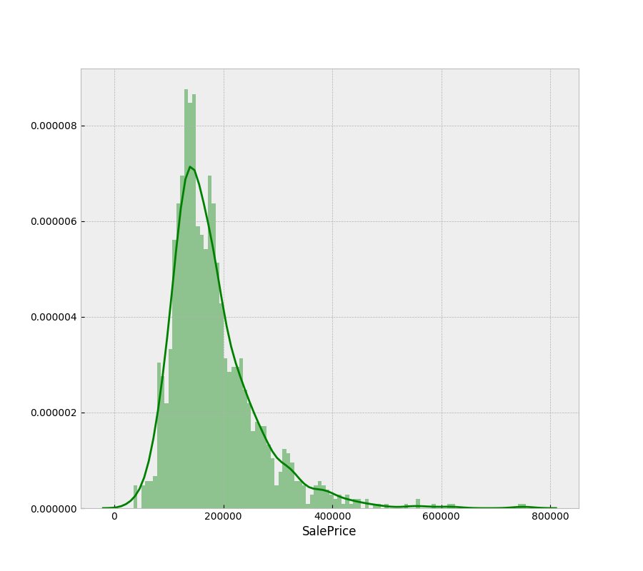
From the above graph we can see that there are very few outliers. Before moving on to the model-building phase, they will be removed.
Now, let us build similar distributions for the other columns and see the relationship they have to sale price.
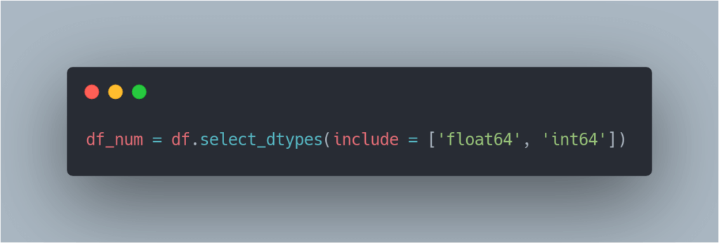
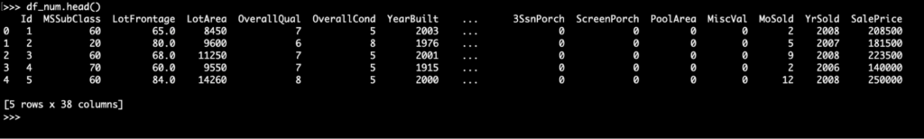
To extract all integer columns:
To plot all of the columns:
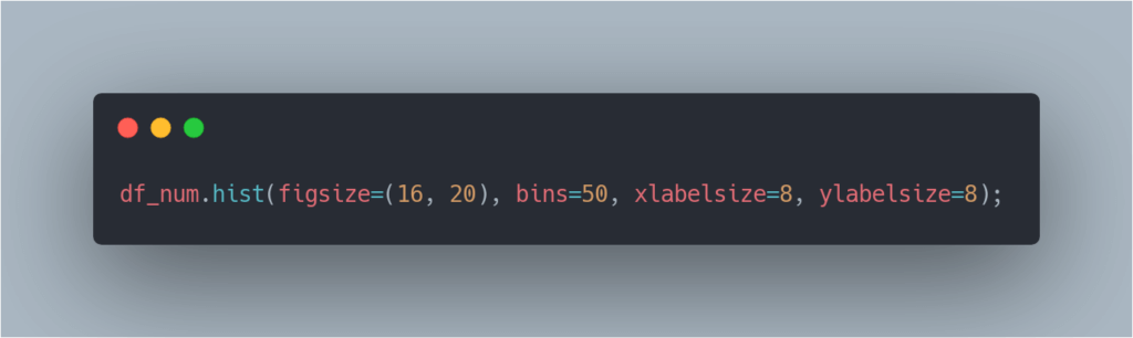
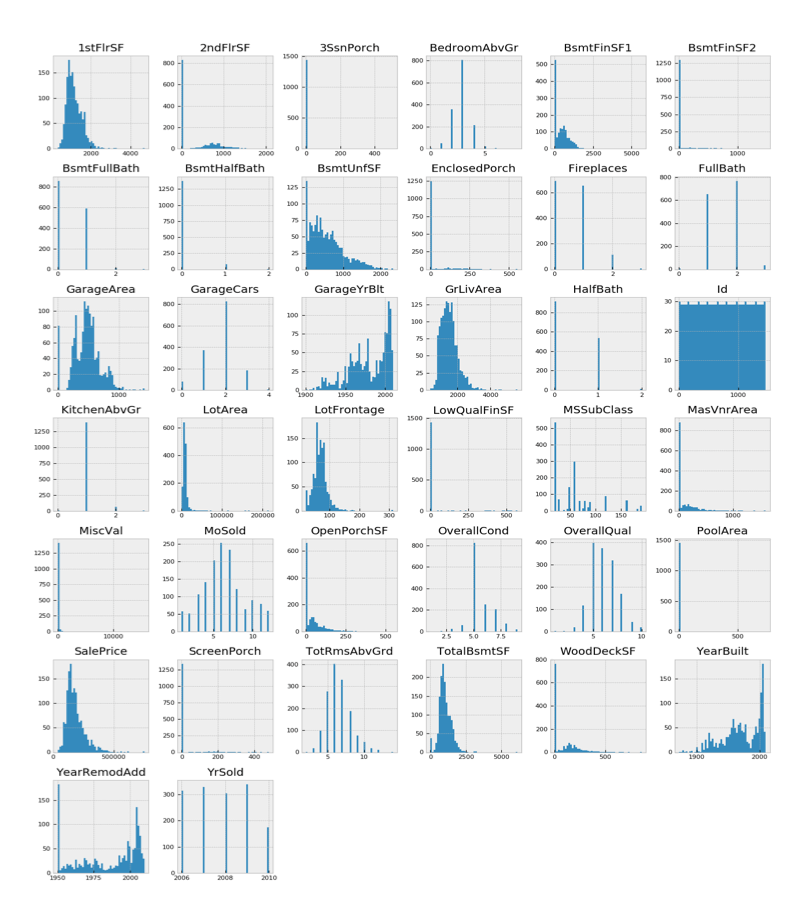
From the above figure, `1stFlrSF`, `TotalBsmtSF`, `LotFrontage`, `GrLiveArea` share a similar distribution to the `SalePrice` distribution. The next step is to uncover correlations between the Xs (house attributes) and the Y (sale price).
Remember folks, correlation is not causation!
Correlations
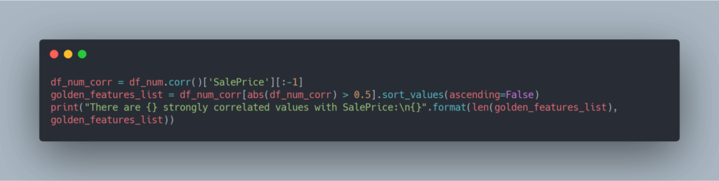
To find those features that have a strong correlation with SalePrice, let’s perform the following:
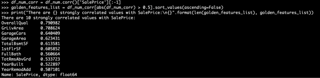
Perfect! We now know there is a strong correlation between these values. This validates the entire dataset, and the effort spent by ML/AI engineers in the next phase should be fruitful.
Now, what about correlations of all the other attributes? It would be too hard to interpret feature-to-feature relationships using distributions. Let’s use a heatmap for this.
Feature to Feature Relationships
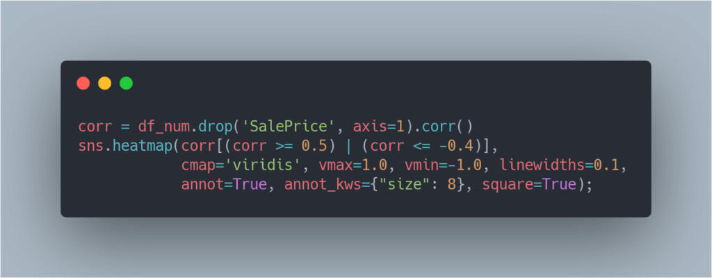
To plot a heatmap between these features, let’s perform the following:
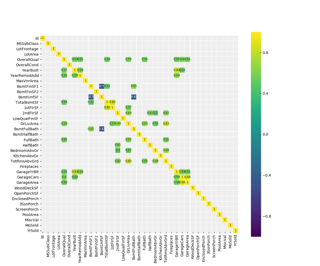
There are a lot of interesting relationships between the features:
- The HalfBath/2ndFlrSF relationship indicates that people give importance to having a half bath on the second floor.
- 1stFlrSF/TotalBsmtSF relationship indicates that the bigger the first floor is, the larger the basement is.
These relationships help us to reconfigure the dataset by removing columns that mean the same thing. This allows us to work with a smaller set of variations, leading to a theoretically higher accuracy.
Conclusion
An ML or AI model can improve significantly if it is pruned and manipulated in the right way. Developers should focus much more time on performing an EDA and then cleaning up the data in order to make building the ML/AI model much easier and more efficient.
All the processes mentioned above can be found on this Github repository.
Related Blogs: