Movie Box Office Data Analysis with Python – Budgets vs Popularity?

When it’s movie night, most of us choose what to watch based on our personal interests first, and popularity second. Popularity is usually based on some viewer or critic ratings database, such as that provided by imdb, rotten tomatoes, metacritic, or similar. But it’s been hypothesized that a film’s budget might actually be a better indicator of popularity rather than critic or viewer ratings. How can we find out? Let’s use Python to do some data analysis and see which is more strongly correlated to popularity: film budgets or ratings.

A Google search for Box Office Data Analysis turns up two public datasets that contain the raw data that we need: 

• Data World Boxoffice mojo has a lifetime box office gross dataset (US only) that also contains the production year for Hollywood movies 
• Kaggle has compiled the ratings and metadata of over 45,000 movies in their Movies dataset, from which we are going to use the movies-metadata.csv.zip file.

Now that we have our data and our goal, we’ll use the following data analysis process to generate our correlations:

1. Install the Movie Correlation Python environment so you can follow along with this tutorial
2. Perform an Exploratory Data Analysis (EDA), which will allow us to quickly get a sense of the data in our datasets
3. Do some Data Cleaning, which will allow us to trim the datasets down to just the data we want
4. Join Two Dataframes, which will allow us to combine the ‘budget’ and ‘ratings’ data
5. Generate Data Correlations, which will help us understand whether/where there’s a significant relationship between our data

Data Analysis Step 1 — Install Python

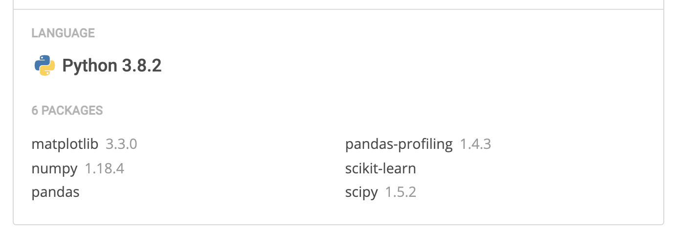
To follow along with the code in this tutorial, you’ll need to have a recent version of Python installed, along with all the packages used in this post. The quickest way to get up and running is to install the Movie Correlation Python environment for Windows or Linux, which contains a version of Python and all the packages you need to follow along with this tutorial, including: 

• Pandas – used to import and clean the data
• pandas-profile – used to perform a quick exploratory data analysis, as well as generate correlations 

In order to download the ready-to-use builds you will need to create an ActiveState Platform account. Just use your GitHub account info to sign up or use your email address. Signing up is very easy! And it unlocks ActiveState Platforms many benefits for you.

For Windows users, run the following at a CMD prompt to automatically download and install our CLI, the State Tool along with the Movie Correlation runtime into a virtual environment:

powershell -Command "& $([scriptblock]::Create((New-Object Net.WebClient).DownloadString('https://platform.activestate.com/dl/cli/install.ps1'))) -activate-default Pizza-Team/Movie-Correlation"

For Linux users, run the following to automatically download and install our CLI, the State Tool along with the Movie Correlation runtime into a virtual environment:

sh <(curl -q https://platform.activestate.com/dl/cli/install.sh) --activate-default Pizza-Team/Movie-Correlation

Data Analysis Step 2 — Exploring Data with Pandas Profiling

A quick exploratory data analysis will give us a first taste of the dimensions, attributes, data types and ranges for each dataset. There are many ways to perform a good EDA, but since we have a clear objective (find the correlation between revenue and budgets or ratings), we are going to rely on an automated EDA tool called pandas profiling. This tool offers a simple way to create an easy-to-read share report from a pandas dataframe.

import hashlib
import pandas as pd
from pandas_profiling import ProfileReport
df_boxoffice = pd.read_csv('./data/boxoffice.csv')
df_metadata = pd.read_csv('./data/movies_metadata.csv.zip')
#simple EDA for boxoffice dataset
eda_boxoffice = ProfileReport(df_boxoffice)
eda_boxoffice.to_file(output_file='./eda/boxoffice_eda.html')
#simple EDA for metadata dataset
eda_metadata = ProfileReport(df_metadata)
eda_metadata.to_file(output_file='./eda/metadata_eda.html')

You can view the output of each file in my GitHub repository under EDA.

Each dataframe contains more information than we require for our simple analysis, so we need to perform some data cleaning before continuing.

Data Analysis Step 3 — Data Cleaning with Lambda Functions

The Boxoffice dataframe contains five columns, from which we need only three: 

• Title
• Lifetime_gross 
• Year

But there are two other problems with this dataset:

• It lacks a simple way to identify a specific movie
• Our automated EDA shows that there are duplicates in the Title column. 

To address these issues, we can use a lambda function to generate a synthetic movie id that identifies each movie uniquely: 

df_boxoffice['id'] = df_boxoffice.apply(lambda x: hashlib.md5(x['title'].replace(" ", "").lower().encode()+str(x['year']).encode()).hexdigest() , axis=1)
del df_boxoffice['rank']
del df_boxoffice['studio']
df_boxoffice

The above code snippet applies a lambda function that calculates the MD5 hash of the string built with the lowercase space-removed ‘title’ of each movie plus the ‘year’ of release, and stores the resulting MD5 string in a new column called ‘id’. After that, the snippet deletes the two unused columns from the dataframe.

Like the Boxoffice dataframe, the Ratings dataframe contains two columns that are not useful for our analysis, so we’ll simply delete them.

Finally, the Metadata dataframe contains 24 columns of data for each movie row, but some of the columns are problematic. For example:

• Our EDA shows that 36,573 movies have a budget of $0 (ie., budget data is not known), which makes them useless for our analysis. We’ll need to remove these rows.
• The ‘id’ and ‘imdb_id’ columns are not related to the synthetic movie id we generated for our Boxoffice dataframe. As a result, we’ll need to build the same synthetic id in this dataframe by extracting the year from the ‘relase_date’ column, and then applying the same lambda function that we used before. The trick here is that our EDA of the ‘release_date’ columns show that there are 87 rows that have no value, so we’ll need to remove those rows before calculating the synthetic id. 

df_metadata.dropna(subset = ['release_date', 'title'], inplace=True)
df_metadata['budget'] = pd.to_numeric(df_metadata['budget'])
df_metadata['year'] = df_metadata.apply(lambda x: str(x['release_date'])[0:4], axis=1)
df_metadata['id'] = df_metadata.apply(lambda x: hashlib.md5(x['title'].replace(" ", "").lower().encode()+str(x['year']).encode()).hexdigest() , axis=1)
df_metadata = (df_metadata.loc[df_metadata['budget'] > 0][['id','title','year','budget','vote_average','vote_count']]).copy()

Data Analysis Steo 4 — Joining Dataframes

As you may expect, we can now combine the two dataframes into a single one. This operation is called a “join.” There are many ways to join two dataframes. In our case, we’re interested in keeping only the rows that exist in both dataframes. To make sure we select only the rows we’re interested in, we’ll use the synthetic ‘id’ field that we created as our key to join on. The resulting dataframe contains 4,309 rows, or nearly 25% of the original Boxoffice dataset.

df = df_metadata.join(df_boxoffice.set_index('id'), on='id', lsuffix='_metadata', rsuffix='_boxoffice')
df.dropna(subset = ['title_boxoffice'], inplace=True)
df.drop_duplicates(subset=['id'], inplace=True)
df

Data Analysis Step 5 — Correlating Movie Data

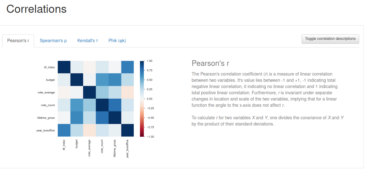
Now that we have a clean dataframe, we can find correlations between columns in several ways. The simplest way is just to use pandas-profiling to perform another EDA of the clean dataframe, since it calculates and plots Pearson’s r, Spearman’s ρ, Kendall’s τ and Phik (φk) correlation types:

#automatic EDA with correlations between vars calculated on the merged dataset
eda_df = ProfileReport(df)
eda_df.to_file(output_file='./eda/df_eda.html')

You may want to open the above graphic in separate tab for greater clarity, but as you can see, the correlations assessment provides us with a heat map matrix showing how each column correlates to every other column in our dataset. For example, Pearson’s r correlation shows: 

• The movie going public pays little attention to reviews (vote_average) when a movie is first released (year_boxoffice) 
• Lifetime box office revenue (lifetime_gross) is strongly correlated to vote_count (i.e., the number of viewers that rated a film), which makes sense if raters also paid to view the movie

Now lets slice the resulting dataset to check whether the movie going public prefers to pay to watch higher budget movies (i.e., blockbusters like superhero or Transformers films) or highly rated ones (such as Academy award winners). 

#select the higher budget and higher rated films
df_hb = df.loc[df['budget'] > 100000000]
df_hr = df.loc[(df['vote_average'] >= 7.5) & (df['vote_count'] > 3)]
#get correlation between budget and box office for hr
print(df_hb['budget'].corr(df_hb['lifetime_gross']))
print(df_hb['vote_average'].corr(df_hb['lifetime_gross']))

For higher budget films, we’ll select movies that have a budget of over $100M. For highly rated films, we’ll include only those movies rated an average of 7.5 or higher (and that have a minimum of 3 votes). The size of the resulting datasets are similar: 288 films vs 292 films. Pearson’s correlation shows roughly a 0.400 correlation of higher budget movies to lifetime box office gross, and a 0.518 correlation for highly rated films. As a result, if you’re a filmmaker, you should be focused on making a good film, rather than an expensive one. 

I’ll leave it to the reader to see if the Spearman’s, Kendall’s or Phik correlations agree with Pearson’s. You can check the complete source code and resulting EDA files in my Github repo.

Conclusions

Note that the film budget data in our dataframe excludes film promotion and marketing, which is the responsibility of the film distributor. If a marketing budget data source could be found, it would be interesting to see how strong a relationship it has to box office gross. As it is, the budget information in this post includes only the cost of script, cast, producer(s), director(s), music, effects and general production costs.

So is budget a better indicator of movie popularity, as measured by box office take? According to our study, a film’s lifetime_gross correlates more strongly to vote_average than budget. Better films make more money!

This post provided a simple example of how to work with heterogeneous datasets. Note that real-world scenarios typically require many more transformations in order to build an analytics-friendly dataset. But no matter how simple or complex, Python provides an amazing set of open source tools to get any job done. 

• Sign up for a free ActiveState Platform account so you can download the Movie Correlation Python environment for Windows or Linux, and see what conclusions you can draw
• View all the code and data in my Movie Box Office Correlation GitHub repository

Related Reads

How to Clean Machine Learning Datasets Using Pandas

Exploratory Data Analysis using Python