Banks are concerned with multiple issues in 2024, not least of which include inflation and a slowing global economy. But these are of far more short term concerns when compared against the ever-growing adoption of technology, which is currently focused on the benefits of Generative AI (GenAI) and the cloud, as well as the threats associated with the digitization of both money and identity.
All of these motions expose the Financial Services (FinServ) industry, including banking, trading and insurance to the risk of cyberattacks at a time when, according to Statista, worldwide losses associated with cybercrimes are expected to top $10T for the first time next year:
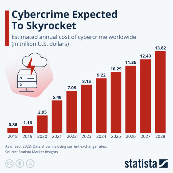
Source = Statista
But FinServ doesn’t really have much of a choice since AI applications are seen as the key to changing everything for the better, from customer service to financial management to back-office operations. In fact, it’s estimated that Artificial Intelligence/Machine Learning (AI/ML) will increase productivity by ~37% as soon as 2025 by simply removing the need for many manual tasks. In other words, despite having spent billions on automating various processes across the transaction lifecycle, humans are still very much in the loop. GenAI apps promise to free up these workers, allowing them to focus on more value-added tasks.
The biggest benefit is likely to come in the form of greater personalization derived from the likes of chatbots that can provide tailored financial planning and custom investment strategies based on customer preferences, as well as their behavioral data. Insurers will also be able to create personalized offerings based on each individual’s risk.
For example:
- Northwestern Mutual, imitating dating apps, created a matchmaking algorithm to pair each customer with their most suitable financial advisor.
- JPMorgan is currently trademarking “IndexGPT,” an app that can perform analysis and select securities based on a client’s profile and their risk preferences.
- HDFC ERGO, an India-based arm of Munich Re, uses AI to provide personalized experiences for customers, from onboarding to issue resolution to claims handling.
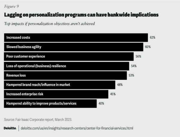
According to Deloitte, those that fail to embrace this wave of personalization via GenAI apps will suffer dramatic consequences:
A balance needs to be struck between the imperative of implementing GenAI apps and the likelihood of being exposed to both ethical and security risks given that all this is occurring in the face of an ongoing AI arms race between cybercriminals, who are leveraging AI in novel ways, and FinServ organizations who are trying to close emerging attack vectors as fast as possible. Cybersecurity is the key.
Here are the top 5 cybersecurity risks associated with AI that FinServ should be planning around and budgeting for in 2024:
1 – Phishing in FinServ
It should be no surprise that phishing is at the top of the list for FinServ, as it is for most industries given that there are ~3.4B phishing emails sent each and every day, which end up being the main catalyst in 93% of all data breaches.
Here, AI should be seen as a two-edged sword: AI-enabled spam filters catch most phishing emails, but AI also provides criminals with a key resource to generate ever more convincing emails designed to fool unsuspecting employees into revealing network login credentials or other confidential information.
While most phishing attempts are sent from an external party and include some information about the target, the most effective ones take the form of reply messages to an existing internal email thread, which can happen if an employee’s email has been hacked. This tactic, known as email conversation thread hijacking, is far more dangerous since it’s harder to recognize as an attack, meaning employees are more likely to click on compromised attachments or links to fake websites.
The solutions have long been understood, including:
- Multifactor Authentication (MFA) – when multiple methods are required for authentication, phishing attempts will need to ask for more specifics, raising suspicion.
- Email Spam Filters – AI-driven detection and blocking of phishing emails is getting better and better, and can typically deflect 99% of attempts.
- Employee Training – awareness of existing and emerging phishing techniques is half the battle, since employees are the primary target.
- IPv6 Email Infrastructure – IPv6 provides better encryption and a greater range of IP addresses, reducing the risk of IP spoofing, which is a common tactic in phishing attacks.
2 – FinServ Vendor Management
Many of the new AI-based applications and technologies FinServ organizations are looking to implement in 2024 will be created and/or managed by partners, raising the profile of security threats associated with vendor risk management. For example, a recent survey sent to wealth managers and private bankers indicated that 72% are planning to partner with FinTechs, broker-dealers, and other custodians to help build out tactical technology infrastructure, thereby freeing up internal resources to focus on strategic initiatives.
The problem lies in the gap between the FinServ industry’s strict regulations around protecting customer data versus third-party vendors who may not be subject to the same restrictions. This gap exposes organizations to a number of risks, including:
- Cybersecurity – because different vendors have different cybersecurity practices, FinServ organizations have a difficult time creating a “one size fits all” security standard they can apply to evaluate the entirety of their vendor base.
- Standardizing on a single AI vendor can simplify alignment with internal guidelines, if possible.
- Operational: third parties that provide and/or manage critical AI services can have a major impact on business continuity when they go down.
- Legally binding SLAs with built-in penalties can help defer risk, but sourcing a secondary, backup vendor (if possible) is the best way to ensure uninterrupted operations.
- Financial: a vendor’s AI-based trading algorithm can expose the organization to financial risk, depending on performance.
- Munich Re offers coverage for AI trading programs that can help mitigate potential financial losses from AI underperformance.
- Compliance: a vendor’s commitment to complying with legislation, regulations and agreements that affect FinServ can be far less stringent than required.
- Legally binding contracts that enforce compliance along with built-in penalties for transgression can help defray risk.
- Reputational: negative public opinion caused by a third party can be significant, especially when it results from third-party data breaches due to poor security controls.
- Where possible, implement continuous monitoring of your third-party’s attack surface to quickly remediate security issues as they’re discovered.
3 – FinServ Vulnerability Management
AI applications, just like all modern software, are primarily built from open source code, which tyipcally forms ~80% of the codebase. While Open Source Software (OSS) vulnerabilities continue to escalate year on year, this is primarily due to the fact that more and more organizations are not only using more OSS, but also reporting vulnerabilities in a more systematic manner.
At the same time, less than half of cybersecurity professionals claim to have high (35%) or complete visibility (11%) into vulnerabilities within their deployed applications. At best, only around half of all organizations (51%) can claim to have moderate visibility into their vulnerabilities.
While FinServ tends to be more proactive about vulnerabilities than non-regulated industries, the key issues remain the same:
- Discoverability – creating a comprehensive catalog of all open source components deployed across the extended enterprise is key to decreasing Mean Time To Identification (MTTI) of vulnerabilities. Software Composition Analysis (SCA) tools are commonly use to automate the catalog creation process (replacing the previous solution of manually populated spreadsheets), but since they essentially reverse engineer a compiled artifact in order to identify all the open source components contained within it, they may be producing an incomplete list. Software Bills Of Material (SBOMs) are no substitute since they are often generated by the same SCA tools.
- While you could generate your catalog from an application’s source code instead, if that source code contains precompiled open source components, you’re no better off. By contrast, ActiveState builds all open source components from source code, including linked C libraries, providing a truly comprehensive SBOM.
- Remediabiility – Mean Time To Exploit (MTTE) has decreased to as little as 22 minutes from the announcement of a vulnerability until the first instance of it’s exploitation in the wild. The lengthy process of investigating a vulnerability, and then patching/upgrading, recompiling, restesting and redeploying the affected application precludes being able to deal with such aggressive cybercriminals. Employing a CI/CD system that features extensive test suites as well as automated deployment to production can help decrease Mean Time To Remediation (MTTR), but not if you have to wait for an upstream OSS patch.
- By comparison, ActiveState continually sources downstream component patches, and rebuilds the affected open source software in minutes ready to be pulled into your CI/CD process for testing and redeployment.
4 – FinServ Malware Threat
Malware (short for malicious software) refers to hacker-created intrusive software designed to steal data, damage computers or compromise computer systems. Traditional malware vectors of attack include phishing, vulnerability exploits, as well as being embedded in the open source components of your software supply chain.
While malware variants are limited only by a cybercriminal’s imagination, the one top of mind for most FinServ organizations is ransomware. Ransomware typically encrypts data across the enterprise, locking users out, but can also exfiltrate that data prior to encryption.
As Sophos’ State of Ransomware in Financial Services 2024 report indicates, FinServ organizations are hit by ransomware attacks at a higher rate (65%) than the cross-industry average (59%), with ransoms averaging $2M. While 51% of FinServ firms pay the ransom to regain access to their data, they may also face demands from the cybercriminal to pay a second ransom in order to prevent leaking the exfiltrated data on the dark web.
Combatting ransomware requires a multi-pronged approach. See the sections above for tactics when it comes to phishing and vulnerabilities. When it comes to building AI applications, attention must be paid to software supply chain attack vectors, where the following best practices apply:
- Automated Code Scanning – open source components should always be scanned using common threat detection tools such as Software Composition Analysis (SCA) for binaries and/or Static Application Security Testing (SAST) for source code.
- Keep in mind that while scanning works well on non-obfuscated code, hackers typically use compression, encryption and other techniques to hide their malware from scanners. Consider using only vetted, securely built and signed open source components from a trusted vendor.
- Dynamic Analysis – Dynamic Application Security Testing (DAST) tools can be successful at catching obfuscated malware when the application is run.
- Care must be taken to not only exercise the code thoroughly, but to do so in an isolated, ephemeral network segment so as to avoid infecting the organization.
- Repositories & Firewalling – a typical FinServ strategy is to deploy an artifact repository from which vetted open source packages are made available to developers. Coupled with firewall blocking of open source repositories (as well as other sites that may pose a risk), this method can be effective in limiting risk.
- Be aware that open source dependencies in artifact repositories can quickly become out of date and vulnerable. FinServ stakeholders must be proactive in approving new versions of dependencies for use, and replacing older versions.
- Signed Code – rather than obtaining open source from public repositories and applying the practices listed above, some FinServ organizations use only open source code that has been securely built and signed by a trusted partner.
- Ensure that artifacts such as Provenance Attestations are collected and maintained as proof of trustworthiness of the components.
5 – FinServ Secure Build Systems
Secure software development best practices extend from developer desktops through code repositories to the CI/CD build system. Each of these environments should be implemented with secure controls to ensure code is being developed, checked in/out and built in a manner that minimizes risk.
Build systems are far too often given short shrift when it comes to security for a number of reasons, not least of which is the complexity of creating a declarative pipeline that allows control over every step of the build process. However, as Solarwinds proved in December 2020, build systems must be hardened to eliminate attack vectors such as the abiliy to inject compromised dependencies into the build process prior to the signing step.
When creating a build system, FinServ organizations should implement a number of best practices, including:
- Hardening – create a dedicated build service that runs on a minimal set of predefined, locked down resources rather than a developer’s desktop or other arbitrary system that can offer a larger attack surface to hackers.
- Automation – execute only scripted builds using scripts that cannot be accessed and modified within the build service, preventing exploits.
- Ephemeral, Isolated Build Steps – every step in a build process must execute in it’s own container, which is discarded at the completion of each step. In other words, containers are purpose-built to perform a single function, reducing the potential for pollution or compromise.
- Hermetic Environments – containers must have no internet access, preventing (for example) dynamic packages from including remote resources.
- Signing – all output artifacts must be digitally signed to ensure they haven’t been tampered with between creation and use.
- Reproducible – all built artifacts must be verified against a hash to ensure that the same “bits” input always result in the same “bits” output.
Conclusions: FinServ vs Cybercriminals
The Financial Service industry is disproportionately targeted by cybercriminals because that’s where the money is. As FinServ rolls out AI applications in 2024, it faces a number of cybersecurity challenges. Whether those applications are built internally or sourced from a partner, security best practices must be proactively put in place to reduce the organization’s exposure to risk.
The quickest way to implement many of these best practices may be to partner with a third party that can more effectively create a scalable secure software supply chain solution – from importing open source components to creating a secure build service to tracking and remediating vulnerabilities – than each FinServ organization can do alone. ActiveState can help.
Next Steps
Watch our Securing AI from Open Source Supply Chain Attacks webinar to learn more about creating and implementing secure AI applications.