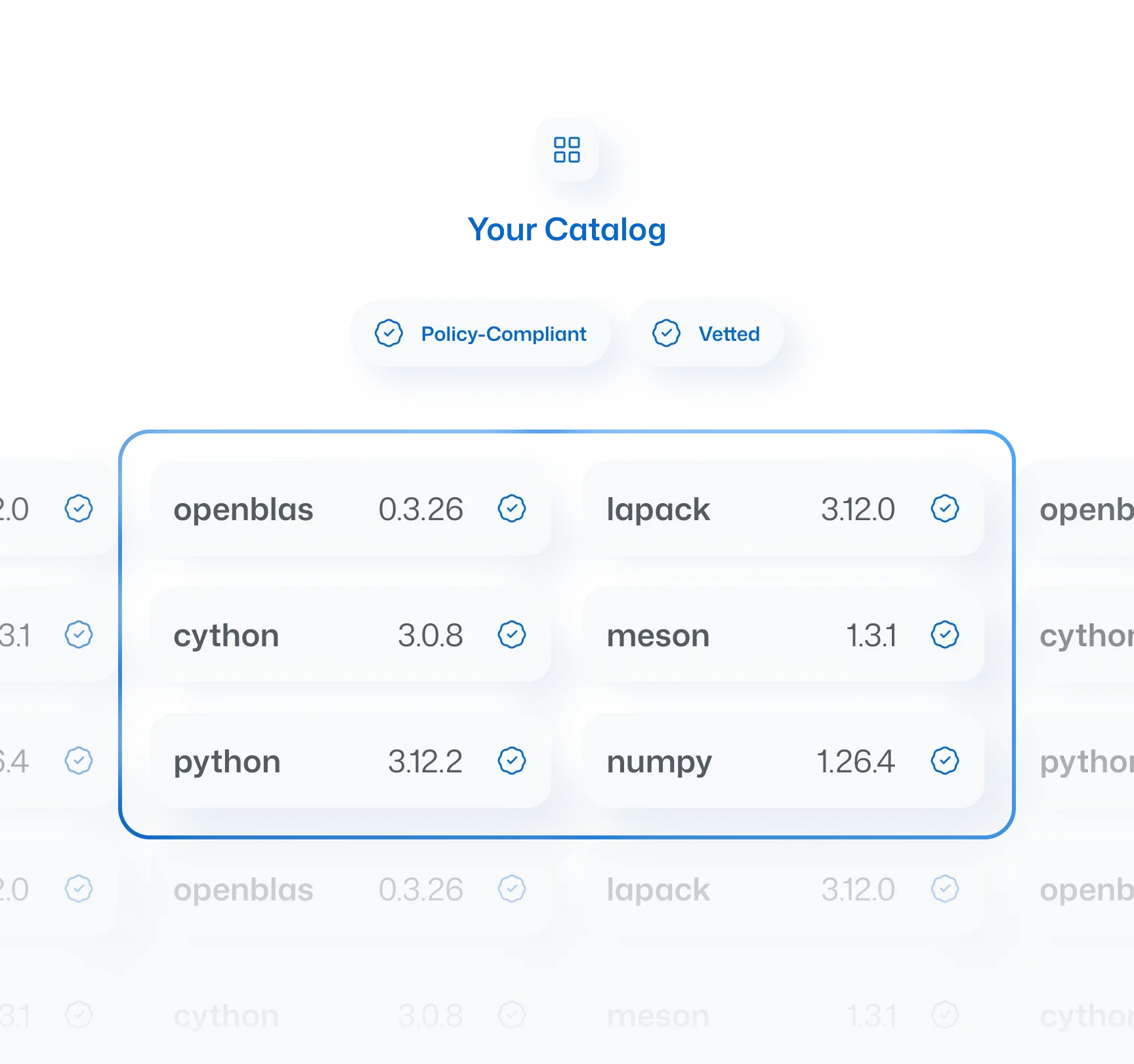
How to Build an Identity Graph with Graph Databases

Today’s businesses and organizations have access to multiple tools for collecting meaningful information about their customers, including:

• Analytics dashboards
• Telemetry
• Access logs

With them they can help identify and portray an accurate picture of their customers’ behavioral patterns.

However, if you’re trying to generate up-to-date, personalized recommendations per customer, such information is simply not good enough. Times are harsh, competition is rising, and customer loyalty is paramount to future profitability, so organizations need to step up their efforts to provide the best customer experience.

You can think of an identity graph (or ID graph) as a database of information that stores both entities and the connections between them. These entities are modeled based on specific characteristics of a business’s requirements and goals. For example:

• In a social network, ID graphs show connections between friends and colleagues
• For a movie subscription platform like Netflix, ID graphs show customer device info or movie recommendations.

All of this information is tied to individual customer IDs so the business can offer personalized experiences and promotions.

We’ve all received an email from Netflix or Amazon Prime recommending movies to watch based on our likes/viewing patterns. This is an example of how ID graphs coupled with machine learning can suggest a list of personalized items to help increase usage time and attract more customers:

One of Many Email Recommendations Netflix Has Sent Me

Creating an ID graph using graph databases is a powerful modern option for linking customer information across platforms without using traditional off-the-shelf services. In this tutorial, we’ll do just that using Python and the following steps:

1. Install a development environment with all the packages we’ll need
2. Model the entities and relationships
3. Populate an identity graph
4. Query an identity graph for a specific user using information like device identifiers, cookies and browsers
5. Update the graph database

Let’s get started.

Step 1 — Install Identity Graph Python Environment

To follow along with the code in this article, you can download and install our pre-built Identity Graph Python environment, which contains:

• A version of Python 3.10.
• All the dependencies used in this post in a pre-built environment for Windows, Mac and Linux:
  • rdflib is a Python library for working with the Resource Description Framework (RDF). This is a standard for representing data in the form of triples (subject-predicate-object), which is useful for representing identity graphs.
  • SPARQLWrapper is a simple Python wrapper around a SPARQL service that helps execute queries remotely. Both of these tools allow us to build nice, robust identity graphs that can be queried using a common language.

In order to download this ready-to-use Python project, you will need to create a free ActiveState Platform account. Just use your GitHub credentials or your email address to register. Signing up is easy and it unlocks the ActiveState Platform’s many other dependency management benefits.

Windows users can install the Face Verification runtime into a virtual environment by downloading and double-clicking on the installer. You can then activate the project by running the following command at a Command Prompt:

state activate --default Pizza-Team/Identity-Graph

For Mac and Linux users, run the following to automatically download, install and activate the Face Verification runtime in a virtual environment:

sh <(curl -q https://platform.activestate.com/dl/cli/_pdli01/install.sh) -c'state activate --default Pizza-Team/Identity-Graph'

Step 2 — Model Definition

The most important part of the process of building an identity graph is to model the different kinds of entities and relationships. Using graph theory terminology, we have:

• Nodes for entities
• Edges for relationships
• Data for related information that we want to capture

Let’s define each one of these in detail:

• Nodes– represent the entities that you want to track in your identity graph. In our case, we need to define the following nodes:

• • User: represents an individual person who accesses the service. We need their id, name, and age.
  • Device: represents a device that a particular person uses to run a browser.
  • Browser: represents the browser application that a particular person uses to access a service.
  • Cookie: represents the cookie data that devices carry as identifiers across devices.

• Edges – represent the relationships between your entities. In our case, we need to define the following connections:

• • Devices & users: users can have one or more associated devices. We just need to create a usedBy relationship field.
  • Cookies & devices: a cookie can be associated with a device. We just need to create a usedOn relationship field.
  • Browsers & devices: a specific browser application can be associated with a device. We just need to create a usedOn relationship field.

• Data Types– in addition to IDs, we need relevant data types that accurately capture the information we want to query in the final graph set. This mainly depends on the amount of data you want to capture and correlate. We’ll just use the ID fields for the sake of simplicity.

Step 3 — Populating the Graph

Based on the model definition work we completed earlier, we can now populate the graph with some data. We will create a small database with:

• 3 users
• 4 browsers
• 6 devices
• A few dozen cookie payloads shared among them

Create a new file in the project directory called data.json and add some user data:

// data.json

{

    "users": [

        {

            "id": "73Wakr",

            "name": "John",

            "age": "32"

        },

        {

            "id": "2OglH6",

            "name": "Joe",

            "age": "39"

        },

        {

            "id": "2Og3J8",

            "name": "Linda",

            "age": "23"

        }

    ],

}

Then, add the following helper functions to a new file named models.py to add them to the graph. Use the following setup code to configure the identity graph:

# models.py

from rdflib import Graph, Namespace, Literal

from rdflib.namespace import RDF

import json


EX = Namespace("http://example.org/")


g = Graph()

g.bind("ex", EX) # bind a custom defined namespace to a prefix

The basic abstraction that we use is the Graph, which represents the container of the nodes, edges, and data. As you can see, we also need to define a custom Namespace to use and bind it as an alias to the exstring. There are other predefined namespaces that are suitable for different use cases (like FriendOfAFriend (FOAF), OWL, SKOS, and PROOF). You can review the list of available namespaces in this section.

Now, add the following helper function to add a new user to the graph:

# Adds a new Person in the graph

def add_person(id, name, age=None):

    person = EX[id]

    g.add((person, RDF.type, EX.Person))

    g.add((person, EX.name, Literal(name)))

    g.add((person, EX.age, Literal(age)))

The most common way to populate the identity graph is to add N-Triples to represent the terms (subject, predicate, and object). For example, in the phrase, “Alex uses iPhone 13”

• The subject is “Alex”
• The predicate is “uses”
• The object is “iPhone 13”

You can read more about the RDF N-Triples spec here.

You can try to test this by loading the JSON file data and printing the graph in this main section:

if __name__ == '__main__':

    with open('data.json', 'r') as f:

        data = json.loads(f.read())

        for user in data['users']:

            add_user(user['name'], user['age'])

    print(g.serialize())


$ python3 models.py

@prefix ex: <http://example.org/> .


ex:2Og3J8 a ex:Person ;

    ex:age "23" ;

    ex:name "Linda" .


ex:2OglH6 a ex:Person ;

    ex:age "39" ;

    ex:name "Joe" .


ex:73Wakr a ex:Person ;

    ex:age "32" ;

    ex:name "John" .

Now you can create similar data files for the rest of the nodes and add them to the graph using the following helper functions:

# Adds a new Device in the graph

def add_device(id, user_id):

    device = EX[id]

    g.add((device, RDF.type, EX.Device))

    g.add((device, EX.usedBy, EX[user_id]))


# Adds a new Browser in the graph

def add_browser(id, device_id):

    browser = EX[id]

    g.add((browser, RDF.type, EX.Browser))

    g.add((browser, EX.usedOn, EX[device_id]))


# Adds a new Cookie in the graph

def add_cookie(id, device_id):

    cookie = EX[id]

    g.add((cookie, RDF.type, EX.Cookie))

    g.add((cookie, EX.usedOn, EX[device_id]))


if __name__ == '__main__':

    with open('data.json', 'r') as f:

        data = json.loads(f.read())

        for user in data['users']:

            add_person(user['id'], user['name'], user['age'])

        for device in data['devices']:

            add_device(device['id'], device['user_id'])

        for browser in data['browsers']:

            add_browser(browser['id'], browser['device_id'])

        for cookie in data['cookies']:

            add_cookie(cookie['id'], cookie['device_id'])

    print(g.serialize(format='turtle'))

This should be enough data to get you started with. We’ll show you how to query the graph next.

Step 4 — Querying the Graph

There are few ways to perform queries. Let’s look at the most common.

Simple Queries by ID

You can perform simple queries for graph data using the value method. If you know the id of the node, you can query relevant fields. For example:

# To get a single value, use ‘value’

id = ’73Wakr’ # User: John

print(g.value(EX[id], EX.name)) # prints: John

print(g.value(EX[id], EX.age)) # prints: 32

print(g.value(EX[id], RDF.type)) # prints: Person

Since we declared the custom EX namespace, it’s important to wrap every property created using the EX[property] or EX.property notation.

Querying Using a SPARQL Server

For most cases, you’ll want to use a SPARQL server to host the graph data and then query it using an SQL-like language. This will allow you to perform complex queries and refine important relationships.

To get started quickly, you can spin up a blazegraph server, which is a graph database that supports RDF/SPARQL APIs:

$ docker run --name blazegraph -d -p 8889:8080 lyrasis/blazegraph:2.1.5

This will create a server running at localhost:8889(which you want to upload the graph). There are multiple ways to populate the remote graph. In this tutorial, we are going to extract the graph into a file that we can upload to the server.

You can export the current graph by adding the following lines at the end of the main method in models.py:

# Save the graph data into a file

g.serialize(destination='example.rdf', format='turtle')

g.close()

Next, navigate to the update path of the SPARQL server endpoint at http://localhost:8889/bigdata/#update and upload the RDF file you just created. You should see a message at the bottom that tells you it was successful.

RDF File Uploaded Successfully

Now, you can perform queries against your RDF graph. We will show you some examples with Python next.

Query for All Users

The following query retrieves the name, age, and ID of all users:

# queries.py

from SPARQLWrapper import SPARQLWrapper, JSON

sparql = SPARQLWrapper("http://localhost:8889/bigdata/sparql")

sparql.setQuery("""

    PREFIX ex: <http://example.org/>

    SELECT ?user ?name ?age

    WHERE {

    ?user a ex:Person ;

            ex:name ?name ;

            ex:age ?age .

    }

""")

sparql.setReturnFormat(JSON)

results = sparql.query().convert()

for result in results['results']['bindings']:

    print(result['user']['value'], result['name']['value'], result['age']['value'])

Running the above script displays the following:

$ python3 queries.py

http://example.org/2Og3J8 Linda 23

http://example.org/2OglH6 Joe 39

http://example.org/73Wakr John 33

Query for a Particular Person’s Device

You can query for devices used by particular people by using the ex:usedBy property. Here’s a sample SPARQL query that returns the devices used by the person with the name “Joe:”

# queries.py

from SPARQLWrapper import SPARQLWrapper, JSON

sparql = SPARQLWrapper("http://localhost:8889/bigdata/sparql")

sparql.setQuery("""

    PREFIX ex: <http://example.org/>

    SELECT ?device

    WHERE {

        ?person ex:name "Joe" .

        ?device ex:usedBy ?person .

    }

""")

sparql.setReturnFormat(JSON)

results = sparql.query().convert()

print("Device List of user: {0}".format('John'))

for result in results['results']['bindings']:

    print("{0}: type={1} value: {2}".format('device', result['device']['type'], result['device']['value']))

Running the above script displays the following:

$ python3 queries.py

Device List of user: John

device: type=uri value: http://example.org/2OglH5

device: type=uri value: http://example.org/2OglKm

device: type=uri value: http://example.org/2OglOi

You can learn more about the SPARQL syntax here.

Step 5 — Updating the Graph

Much like querying, there are multiple ways to update the graph database. Let’s look at some of the most common ways.

Single Updates by ID

You can perform direct updates of graph data using the set method. If you know the id of the node, you can update the relevant fields:

# To change a single of value, use 'set'

id = '73Wakr' # User: John

g.set((EX[id], EX.age, Literal(33)))

print(g.value(EX[id], EX.age)) # prints: 33

Updates Using SPARQL

You can use INSERT DATA to insert new triplets or DELETE DATA to delete specific triplets from the storage. If you are using rdflib to construct an in-memory representation of an identity graph, it’s important to create a SPARQLUpdateStore to keep those operations in sync:

from rdflib.plugins.stores.sparqlstore import SPARQLUpdateStore

import json


EX = Namespace("http://example.org/")

endpoint_url = "http://127.0.0.1:8889/bigdata/sparql"

store = SPARQLUpdateStore(query_endpoint=endpoint_url, update_endpoint=endpoint_url)

Now, instead of saving the graph in a file and uploading it to the store, the SPARQLUpdateStore wrapper will take care of those operations as soon as you perform updates in the graph instance.

Conclusions – Python Identity Graphs Simplify User Profiling

In this tutorial, we explained what an identity graph is and showed you how to build one with Python using rdflib. Creating a custom-made identity graph allows businesses to accurately capture meaningful data about their customers, and then leverage the power of graph databases and semantic structures to correlate the information with high performance and scalability.

You can also perform elaborate, semantically complex queries using SPARQL, which enables you to use a familiar SQL syntax and supporting extensions for geolocation and full-text search if needed.

If you’d like to consult additional resources related to building identity graphs, we recommend the following:

• Apache Jena – SPARQL Tutorial
• AWS Database Blog – “Building a customer identity graph with Amazon Neptune”

Read Similar Stories