
The first step in any machine learning project is typically to clean your data by removing unnecessary data points, inconsistencies and other issues that could prevent accurate analytics results. Data cleansing can comprise up to 80% of the effort in your project, which may seem intimidating (and it certainly is if you attempt to do it by hand), but it can be automated.
In this post, we’ll walk through how to clean a dataset using Pandas, a Python open source data analysis library included in ActiveState’s Python. All the code in this post can be found in my Github repository.
Installing Python and Pandas
If you already have Python installed, you can skip this step. However for those who haven’t, read on!
For this tutorial, I will be using ActiveState’s Python. There’s no major difference between the open source version of Python and ActiveState’s Python – for a developer. However, ActiveState Python is built from vetted source code and is regularly maintained for security clearance.
For this tutorial, you have two choices:
1. Download and install the pre-built “Cleaning Datasets” runtime environment for CentOS 7, or
2. If you’re on a different OS, you can automatically build your own custom Python runtime with just the packages you’ll need for this project by creating a free ActiveState Platform account, after which you will see the following image:

3. If you click the Get Started button you can choose Python, the OS you are working in, and then add “pandas” and “scikit-learn” from the list of packages available.
4. Once the runtime builds, you can you can download the State Tool and use it to install your runtime:
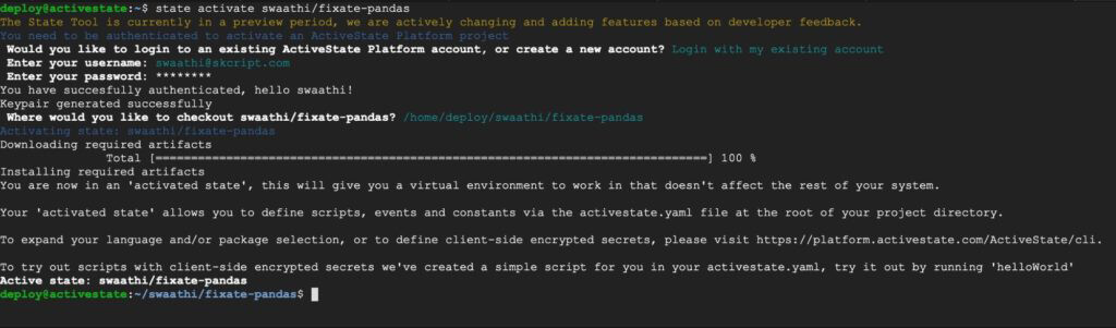
And that’s it! You now have Python installed with all the required packages in a virtual environment. If you want to read a more detailed guide on how to install ActivePython on Linux, please read here.
In this directory, create your first “clean-with-pandas.py” file.
Getting Started with Pandas
The first step is to import Pandas into your “clean-with-pandas.py” file
import pandas as pd
Pandas will now be scoped to “pd”. Now, let’s try some basic commands to get used to Pandas.
To create a simple series (array) on Pandas, just do:
s = pd.Series([1, 3, 5, 6, 8])
This creates a one-dimensional series.
0    1.0
1    3.0
2    5.0
3    6.0
4    8.0
dtype: float64
In most machine learning scenarios, data is presented to you in a CSV file. The great thing about Pandas is that it supports reading and analyzing this kind of data out of the box. Here’s how to read data from a CSV file.
df = pd.read_csv('data.csv')
A typical machine learning dataset has a dozen or more columns and thousands of rows. To quickly display data, you can use the Pandas “head” and “tail” functions, which respectively show data from the top and the bottom of the file:
df.head()
df.tail(3)
You can either pass in the number of rows to view as an argument, or Pandas will show 5 rows by default.
At any time, you can also view the index and the columns of your CSV file:
df.index
df.columns
Choosing a Dataset
For the purpose of this tutorial, we will be using a CSV file containing a list of import shipments that have come to a port. You can find it on the Github repository mentioned here. The file includes attributes of the shipment, as well as whether the shipment was “valid” or not, where valid means officers let the shipment through.
A quick look at the dataset using “df.columns” shows:
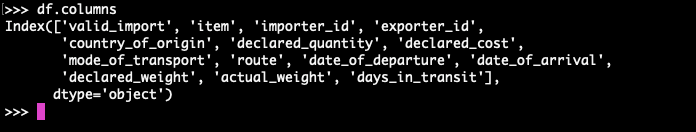
You can explore the dataset further by looking at the number of features, number of rows, the datatype of each column, and so on.
Cleaning A Dataset
Dropping Unnecessary Columns
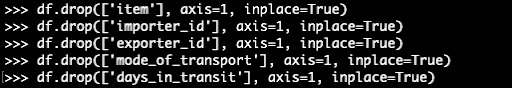
A useful dataset is one that has only relevant information in it. As the first step of the data cleaning process, let’s drop columns that:
- Are not aligned to the dataset goals. From a practical point of view, a dataset may contain data that is irrelevant to the study being undertaken. However, you don’t want to drop data that may actually be useful. Only drop it if you’re sure it won’t be helpful. In this case, “item,” “importer_id” and “exporter_id” can all be dropped from our dataset.
- Have a significant number of empty cells. If a variable is missing 90% of its data points, then it’s probably wise to just drop it all together.
- Contain non-comparable values. Oftentimes datasets contain IDs that are not significant from a data perspective. In other words, they cannot be compared or manipulated mathematically. For this reason, we’ll drop “mode_of_transport.”
On Hot Encoding Labels
The dataset provides routes taken by each shipment. Points along the routes are described using labels, as shown below:
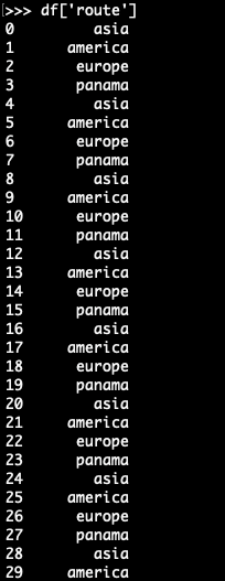
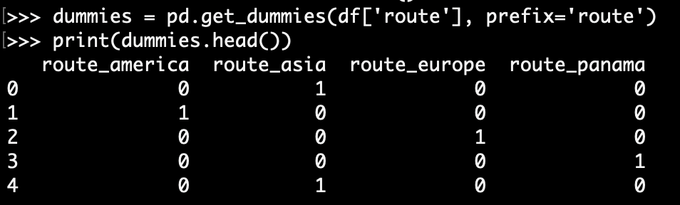
Sending route data to a mathematical model in this form has little value. The data first needs to be represented in a numerically comparable way. For example, “asia” and “america” represent two different locations and cannot be represented in the same column. To solve this, we will create a new column for each unique value in the “route” column. This is automatically done by the “get_dummies” function of Pandas:
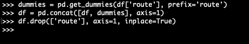
Now the “route” column is no longer necessary. We will drop the “route” column and concatenate the original data with the new columns from the “get_dummies” function.
Repeat this for the “country_of_origin” column as well.
Summarizing Columns
Multiple columns can sometimes convey the same information. In our dataset, “date_of_departure”, “date_of_arrival” and “days_in_transit” all mean the same thing. Additionally, date fields don’t carry much relevance unless represented in a quantifiable way. For this reason, we’ll keep the “days_in_transit” column and drop the two date fields.
Normalizing Quantities
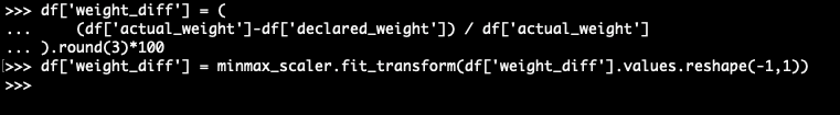
There are two columns that represent the weight of the shipment: “actual_weight” and “declared_weight.” Any shipment that has a large deviation between these two values could potentially be misdeclared. However, a “heavier” shipment will have a larger deviation than a “lighter” shipment. To normalize these values, we’ll use a scaler from the scikit-learn library.
Handling Missing Values
Apart from handling irrelevant columns, it is also important to handle missing values for the columns we actually need. There are multiple ways to go about this:
- Fill in the missing rows with an arbitrary value: can be performed when there is a known default value that doesn’t corrupt the entire dataset
- Fill in the missing rows with a value computed from the data’s statistics: if possible, a better option than number one
- Ignore missing rows: only works if the dataset is large enough to afford throwing away some of the rows
Formatting The Data
Oftentimes datasets are created by humans manually keying in every data point, which is prone to human errors or glitches. For example, a route that goes through the Panama Canal can be represented as “panama” or “Panama Canal” or “panama-canal”. In order to standardize how the Panama Canal appears in the dataset, use the Pandas “replace” function to replace all non-standardized representations.
Conclusion
A machine learning or AI model can improve significantly if it is trained on the right dataset. In most cases, cleaning data and representing it in a mathematically consumable way leads to higher accuracy rates than just changing the model itself. Though there is no rule-of-thumb when it comes to cleaning data, you should always aim for a dataset that is quantifiable, comparable, and has significant relevance to your output.
- To view all the code and processes mentioned in this post, you can refer to my Github repository.
- To run the code, you can sign up for a free ActiveState Platform account and either build your own runtime environment or download the pre-built “Cleaning Datasets” runtime.
Related Blogs: