The success in professional baseball has led to the use of analytics in other professional sports, including hockey, golf, and football. Unsurprisingly, it has also spread to those that bet on the same professional sports. If statistics can be used internally by teams to enhance their win probability, there’s no reason why external observers cannot use the same statistics to determine which team has a higher probability of winning.
Machine learning provides a more advanced toolbox than the sports analytics used previously. When the vast amounts of publicly available sports data is combined with today’s desktop computational power, anyone with an interest in building their own sports betting models can do so. Python is an excellent place to start learning how. Whether your motivation is sports betting, learning Python, or advancing your machine learning expertise, this tutorial is for you.
In this blog post, I will guide you through the steps to create a predictive algorithm using common machine learning techniques:
- Installing Python
- Selecting Data
- Importing and cleaning raw data
- Feature engineering
- Creating a test and training set
- Assessing different machine learning models
- Making predictions
Since the 2020-2021 NFL season is currently about halfway through, it provides an intriguing and relevant source of data upon which we can build our models.
1 – Installing Python for Predicting NFL Games
To follow along with the code in this tutorial, you’ll need to have a recent version of Python installed. The quickest way to get up and running is to install the NFL Game Predictions Python environment for Windows or Linux, which contains a version of Python and all the packages you need to follow along with this tutorial, including:
- Pandas – used to import and clean the data
- Numpy – used to create arrays of data
- Scikit-learn – used to train the model
- Sportsreference package – used to pull NFL data from www.sports-reference.com. The website hosts sports statistics for a myriad of professional sports, and is kept up-to-date as games are played.
For Windows users, run the following at a CMD prompt:
powershell -Command "& $([scriptblock]::Create((New-Object Net.WebClient).DownloadString('https://platform.www.activestate.com/dl/cli/install.ps1'))) -activate-default Pizza-Team/NFL-Game-Prediction-Win"
For Linux users, run the following:
sh <(curl -q https://platform.www.activestate.com/dl/cli/install.sh) --activate-default Pizza-Team/NFL-Game-Prediction
All of the code in this tutorial can be found on my GitLab repository here.
All set? Let’s get started.
2 – Selecting NFL Data to Model
When creating a model from scratch, it is beneficial to develop an approach strategy that clearly delineates the goal of the model. Doing so clarifies which data should be used, how to manipulate the data to construct a training set, and where to obtain the data. Because our goal is to predict the outcomes of NFL games in the 2020-2021 season, the first thing we need to define is the statistical metrics that can best determine whether a team wins or not:
- Obvious in-game metrics include the average amount of points a team scores and the average amount of points a team gives up to the opposing team.
- Less obvious metrics include total number of yards gained and total ball possession time
- Offensive success metrics would include third- and fourth-down conversion efficiency and the number of turnovers
Our model should include all these in-game statistics, among others.
In addition to the standard in-game statistics, we can use external metrics within the model. There are many third-parties that construct their own metrics based on the same in-game statistics, qualitative rankings from experts, historical team rankings that go back decades, and even the exact players that are on the field during each game. Some of these include:
- Nate Silver’s 538 Elo rating
- The Massey Ratings
- NFL Expert Picks, which provide the odds used in Vegas sports betting
Each has its own methodology, but all have been proven successful at predicting game outcomes. Our model should incorporate one or more of these external metrics.
Our approach is to construct a dataset where each row represents a single game between two teams, and the columns are based on the aforementioned metrics. The result of each game is given by either a 0 (for a home team victory) or a 1 (for an away team victory). We can use logistic regression to make a prediction (a probability between 0 and 1) of the away team winning or losing.
Because the 2020-2021 season is only half-way through, it is interesting to see if we can build a model using the games that have already been played to predict the games that will be played in the remainder of the regular season.
3 – Cleaning NFL Data
To obtain the data for the 2020-2021 season, we first need to import the sportsreference package. We’ll use two class methods: Boxscore and Boxscores. The former gives the statistical information for a given game, while the latter provides the game information (teams playing and who wins if the game has already been played). We could easily include data from previous NFL seasons in our model, but to keep the total dataset size and training time down, we’ll include only data from the current season.
It is also worth noting that the nature of the NFL changes from year to year. This year’s league is dominated by quarterbacks that not only pass for a record number of yards, but also that are mobile and accrue rushing yards that often play a critical role in whether a team wins or not. As a result, the weights corresponding to each feature in our model can differ from season to season.
For more information on how to use the sportsreference package, refer to its documented capabilities. To see how these methods work in practice:
from sportsreference.nfl.boxscore import Boxscores, Boxscore
Boxscores(1,2020).games
The first argument is the week of the NFL season (week 1), and the second is the season itself (2020 season). You should see something like this:
{'1-2020': [{'boxscore': '202009100kan',
   ‘away-name’: ‘Houston Texans’,
   ‘away_abbr’: ‘htx’,
   ‘away_score’: 20,
   ‘home_name’: ‘Kansas City Chiefs’,
   ‘home_abbr’: kan’,
   ‘home_score’: ‘34’,
   ‘winning _name’: ‘Kansas City Chiefs’,
   ‘winning _abbr’: ‘kan’,
   ‘losing _name’: ‘Houston Texans’,
   ‘losing _abbr’: ‘htx’,},
  {‘boxscore’: ‘20200913buf’,
   ‘away_name’: ‘New York Jets’,
   ‘away_abbr’: ‘nyj’,
The first game listed is between the Houston Texans and the Kansas City Chiefs, with the Chiefs winning 34 to 20. The first entry in the dictionary is a unique game string. We can use the game string given by boxscore to obtain the statistics for the game:
game_str = Boxscores(1,2020).games['1-2020'][0]['boxscore']
game_stats = Boxscore(game_str)
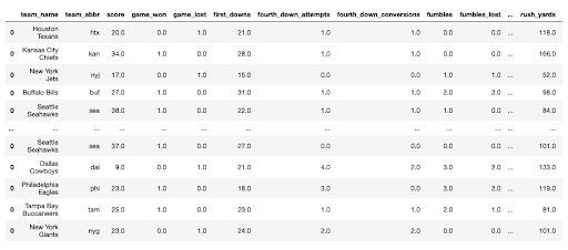
game_stats.dataframe
You should see a dataframe like this:

There are 58 columns worth of statistics in the dataframe. Once a game is played, this dataframe is populated. If a game has not been played, an empty object is returned. The column names can be listed by running:
game_stats.dataframe.columns
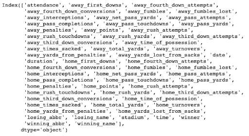
That’s quite a bit of useful statistics from the game! To create our dataset, we’ll need to:
- Loop through all the games that have been played
- Extract the game statistics for each team
- Aggregate the team’s statistics over all previously played games to predict the outcome of the next game.
We also need to extract the schedule, so we know which teams are playing in the coming weeks. This is perhaps the easiest place to start. We can write a function that loops over each week, and each game within each week, to extract the schedule:
def get_schedule(year):
    weeks = list(range(1,18))
    schedule_df = pd.DataFrame()
    for w in range(len(weeks)):
        date_string = str(weeks
for g in range(len(week_scores.games[date_string])):
game = pd.DataFrame(week_scores.games[date_string][g], index = [0])[[‘away_name’, ‘away_abbr’,’home_name’, ‘home_abbr’,’winning_name’, ‘winning_abbr’ ]]
game[‘week’] = weeks
week_games_df = pd.concat([week_games_df,game])
schedule_df = pd.concat([schedule_df, week_games_df]).reset_index().drop(columns = ‘index’)
return schedule_df
From here, we can extract the statistics from each game, using a similar methodology to the get_schedule() function above: define a function that loops through each game, and each week. We also need to manipulate the raw data a bit by dropping columns we don’t need, and transforming others into a more workable format: This function takes the year of the season as input, and returns a dataframe of the games being played each week. This dataframe provides the basis for our final dataset, as each row corresponds to a game.
def game_data(game_df,game_stats):
    try:
        away_team_df = game_df[['away_name', 'away_abbr', 'away_score']].rename(columns = {'away_name': 'team_name', 'away_abbr': 'team_abbr', 'away_score': 'score'})
        home_team_df = game_df[['home_name','home_abbr', 'home_score']].rename(columns = {'home_name': 'team_name', 'home_abbr': 'team_abbr', 'home_score': 'score'})
        try:
            if game_df.loc[0,'away_score'] > game_df.loc[0,'home_score']:
                away_team_df = pd.merge(away_team_df, pd.DataFrame({'game_won' : [1], 'game_lost' : [0]}),left_index = True, right_index = True)
                home_team_df = pd.merge(home_team_df, pd.DataFrame({'game_won' : [0], 'game_lost' : [1]}),left_index = True, right_index = True)
            elif game_df.loc[0,'away_score'] < game_df.loc[0,'home_score']:
                away_team_df = pd.merge(away_team_df, pd.DataFrame({'game_won' : [0], 'game_lost' : [1]}),left_index = True, right_index = True)
                home_team_df = pd.merge(home_team_df, pd.DataFrame({'game_won' : [1], 'game_lost' : [0]}),left_index = True, right_index = True)
            else:
                away_team_df = pd.merge(away_team_df, pd.DataFrame({'game_won' : [0], 'game_lost' : [0]}),left_index = True, right_index = True)
                home_team_df = pd.merge(home_team_df, pd.DataFrame({'game_won' : [0], 'game_lost' : [0]}),left_index = True, right_index = True)
        except TypeError:
                away_team_df = pd.merge(away_team_df, pd.DataFrame({'game_won' : [np.nan], 'game_lost' : [np.nan]}),left_index = True, right_index = True)
                home_team_df = pd.merge(home_team_df, pd.DataFrame({'game_won' : [np.nan], 'game_lost' : [np.nan]}),left_index = True, right_index = True)
        away_stats_df = game_stats.dataframe[['away_first_downs', 'away_fourth_down_attempts',
               'away_fourth_down_conversions', 'away_fumbles', 'away_fumbles_lost',
               'away_interceptions', 'away_net_pass_yards', 'away_pass_attempts',
               'away_pass_completions', 'away_pass_touchdowns', 'away_pass_yards',
               'away_penalties', 'away_points', 'away_rush_attempts',
               'away_rush_touchdowns', 'away_rush_yards', 'away_third_down_attempts',
               'away_third_down_conversions', 'away_time_of_possession',
               'away_times_sacked', 'away_total_yards', 'away_turnovers',
               'away_yards_from_penalties', 'away_yards_lost_from_sacks']].reset_index().drop(columns ='index').rename(columns = {
               'away_first_downs': 'first_downs', 'away_fourth_down_attempts':'fourth_down_attempts',
               'away_fourth_down_conversions':'fourth_down_conversions' , 'away_fumbles': 'fumbles', 'away_fumbles_lost': 'fumbles_lost',
               'away_interceptions': 'interceptions', 'away_net_pass_yards':'net_pass_yards' , 'away_pass_attempts': 'pass_attempts',
               'away_pass_completions':'pass_completions' , 'away_pass_touchdowns': 'pass_touchdowns', 'away_pass_yards': 'pass_yards',
               'away_penalties': 'penalties', 'away_points': 'points', 'away_rush_attempts': 'rush_attempts',
               'away_rush_touchdowns': 'rush_touchdowns', 'away_rush_yards': 'rush_yards', 'away_third_down_attempts': 'third_down_attempts',
               'away_third_down_conversions': 'third_down_conversions', 'away_time_of_possession': 'time_of_possession',
               'away_times_sacked': 'times_sacked', 'away_total_yards': 'total_yards', 'away_turnovers': 'turnovers',
               'away_yards_from_penalties':'yards_from_penalties', 'away_yards_lost_from_sacks': 'yards_lost_from_sacks'})
         home_stats_df = game_stats.dataframe[['home_first_downs', 'home_fourth_down_attempts',
               'home_fourth_down_conversions', 'home_fumbles', 'home_fumbles_lost',
               'home_interceptions', 'home_net_pass_yards', 'home_pass_attempts',
               'home_pass_completions', 'home_pass_touchdowns', 'home_pass_yards',
               'home_penalties', 'home_points', 'home_rush_attempts',
               'home_rush_touchdowns', 'home_rush_yards', 'home_third_down_attempts',
               'home_third_down_conversions', 'home_time_of_possession',
               'home_times_sacked', 'home_total_yards', 'home_turnovers',
               'home_yards_from_penalties', 'home_yards_lost_from_sacks']].reset_index().drop(columns = 'index').rename(columns = {
               'home_first_downs': 'first_downs', 'home_fourth_down_attempts':'fourth_down_attempts',
               'home_fourth_down_conversions':'fourth_down_conversions' , 'home_fumbles': 'fumbles', 'home_fumbles_lost': 'fumbles_lost',
               'home_interceptions': 'interceptions', 'home_net_pass_yards':'net_pass_yards' , 'home_pass_attempts': 'pass_attempts',
               'home_pass_completions':'pass_completions' , 'home_pass_touchdowns': 'pass_touchdowns', 'home_pass_yards': 'pass_yards',
               'home_penalties': 'penalties', 'home_points': 'points', 'home_rush_attempts': 'rush_attempts',
               'home_rush_touchdowns': 'rush_touchdowns', 'home_rush_yards': 'rush_yards', 'home_third_down_attempts': 'third_down_attempts',
               'home_third_down_conversions': 'third_down_conversions', 'home_time_of_possession': 'time_of_possession',
               'home_times_sacked': 'times_sacked', 'home_total_yards': 'total_yards', 'home_turnovers': 'turnovers',
               'home_yards_from_penalties':'yards_from_penalties', 'home_yards_lost_from_sacks': 'yards_lost_from_sacks'})
         away_team_df = pd.merge(away_team_df, away_stats_df,left_index = True, right_index = True)
        home_team_df = pd.merge(home_team_df, home_stats_df,left_index = True, right_index = True)
        try:
            away_team_df['time_of_possession'] = (int(away_team_df['time_of_possession'].loc[0][0:2]) * 60) + int(away_team_df['time_of_possession'].loc[0][3:5])
            home_team_df['time_of_possession'] = (int(home_team_df['time_of_possession'].loc[0][0:2]) * 60) + int(home_team_df['time_of_possession'].loc[0][3:5])
        except TypeError:
            away_team_df['time_of_possession'] = np.nan
            home_team_df['time_of_possession'] = np.nan
    except TypeError:
        away_team_df = pd.DataFrame()
        home_team_df = pd.DataFrame()
    return away_team_df, home_team_df
This function does a number of things:
- Defines two dataframes: one for the home team, and one for the away team.
- For each dataframe, it creates columns for game_won and game_lost, which are populated with either a 0 (loss) or 1 (win). If there is a tie (which has occurred this season, in week 3), neither team gets a win or loss. The win/loss/tie data is taken from the Boxscores method.
- Appends the game statistics from the Boxscore method onto each respective team, and renames the columns, such that all teams have identically named features.
- Modifies the time_of_possession column to be expressed in a single unit of time (seconds instead of minutes:seconds).
With this function, we can write an additional function that loops through each week and game, extracting the game statistics for each team using the game_data function:
def game_data_up_to_week(weeks,year):
    weeks_games_df = pd.DataFrame()
    for w in range(len(weeks)):
        date_string = str(weeks
4 – Feature Engineering – Defining NFL Win/Loss Criteria
Thus far we have written functions that allow for the extraction of the NFL schedule, along with the in-game statistics of the games that have been played. In order to construct a model, we now need to transform the statistics for each game into “features” we can use to train a model.
A “feature” reflects how each team has performed in the weeks preceding the current game. So, for example, if a game is played in week 6 between the Tennessee Titans and the Houston Texans, the features should represent how the Tennessee Titans and Houston Texans have performed in weeks 1 through 5.
To create these features, we’ll define the agg_weekly_data() function, which aggregates each team’s statistics up to the week in question. So for the games in week 2, the statistics are solely given by the week 1 results. For the week 3 games, the statistics are the average results from weeks 1 and 2. This implies that a team’s average statistics will change from week to week, but will all be included in the final dataset that we use to train our model.
def agg_weekly_data(schedule_df,weeks_games_df,current_week,weeks):
    schedule_df = schedule_df[schedule_df.week < current_week]
    agg_games_df = pd.DataFrame()
    for w in range(1,len(weeks)):
        games_df = schedule_df[schedule_df.week == weeks
-
- Loops through each week up to the week in question
-
- Sums those statistics that need to be summed – such as wins and losses – across each week
-
- Averages the remaining statistics over the weeks (such as total yards in each game, points per game, etc.)
-
- Combines a few of the features:
-
- Wins and losses are combined to win percentage
-
- Third- and fourth-down conversions and attempts are combined to third- and fourth-down conversion percentage
-
- Combines a few of the features:
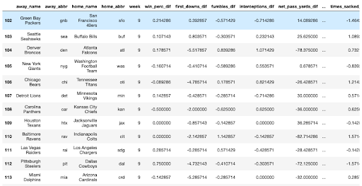
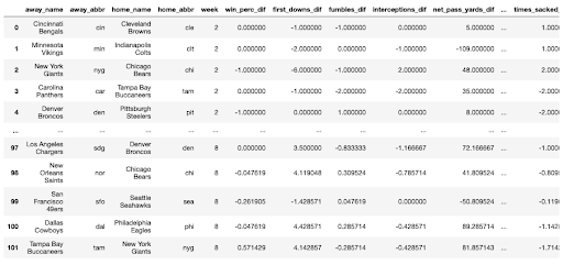
For each game in question, this process of aggregation is done for both the away and home team, then merged onto each respective team. To keep things clear, we add a prefix onto the column names: away_ for the away team, and home_ for the home team. Following this, we calculate the differential statistics between each team. So, pass_yards_dif is the difference between away_pass_yards and home_pass_yards. For our model to be able to predict which team wins, we need features that represent differential performance between the teams, rather than absolute statistics for each team in separate columns. If a game has not yet occurred (e.g. predict week 12 game outcomes when only games up to week 9 have occurred), we skip over these statistics, and add in a message indicating that these games have not occurred yet. The final dataframe should look like the following: 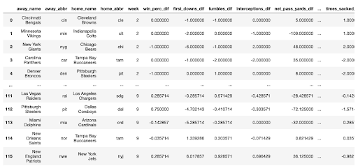
5 – Modeling NFL Rankings
Now that we have aggregated all the in-game statistics we want to use, we can move on to adding external metrics by including Nate Silver’s 538 Elo rating. The rating is essentially a power rating for each team, based on their historical head-to-head results. This includes not only games from the current season but all previous seasons. But in addition to the power rating, they also include a few corrections, including a correction for the quarterback playing in each game. As the most important position in football, the quarterback plays a critical role in the outcome of any given game. For example, injuries to a team’s best quarterback can heavily influence the probability of winning. As expected, 538 ratings vary from game to game, especially if there is a change in quarterback. We’ll include two of the 538 ratings: raw power rating and individual quarterback rating. To extract these ratings, we’ll define the get_elo() function as follows:
def get_elo():
    elo_df = pd.read_csv('nfl_elo_latest.csv')
    elo_df = elo_df.drop(columns = ['season','neutral' ,'playoff', 'elo_prob1', 'elo_prob2', 'elo1_post', 'elo2_post',
           'qbelo1_pre', 'qbelo2_pre', 'qb1', 'qb2', 'qb1_adj', 'qb2_adj', 'qbelo_prob1', 'qbelo_prob2',
           'qb1_game_value', 'qb2_game_value', 'qb1_value_post', 'qb2_value_post',
           'qbelo1_post', 'qbelo2_post', 'score1', 'score2'])
    elo_df.date = pd.to_datetime(elo_df.date)
    elo_df = elo_df[elo_df.date < '01-05-2021']
    elo_df['team1'] = elo_df['team1'].replace(['KC', 'JAX', 'CAR', 'BAL', 'BUF', 'MIN', 'DET', 'ATL', 'NE', 'WSH',
           'CIN', 'NO', 'SF', 'LAR', 'NYG', 'DEN', 'CLE', 'IND', 'TEN', 'NYJ',
           'TB', 'MIA', 'PIT', 'PHI', 'GB', 'CHI', 'DAL', 'ARI', 'LAC', 'HOU',
           'SEA', 'OAK'],
            ['kan','jax','car', 'rav', 'buf', 'min', 'det', 'atl', 'nwe', 'was',
            'cin', 'nor', 'sfo', 'ram', 'nyg', 'den', 'cle', 'clt', 'oti', 'nyj',
             'tam','mia', 'pit', 'phi', 'gnb', 'chi', 'dal', 'crd', 'sdg', 'htx', 'sea', 'rai' ])
    elo_df['team2'] = elo_df['team2'].replace(['KC', 'JAX', 'CAR', 'BAL', 'BUF', 'MIN', 'DET', 'ATL', 'NE', 'WSH',
           'CIN', 'NO', 'SF', 'LAR', 'NYG', 'DEN', 'CLE', 'IND', 'TEN', 'NYJ',
           'TB', 'MIA', 'PIT', 'PHI', 'GB', 'CHI', 'DAL', 'ARI', 'LAC', 'HOU',
           'SEA', 'OAK'],
            ['kan','jax','car', 'rav', 'buf', 'min', 'det', 'atl', 'nwe', 'was',
            'cin', 'nor', 'sfo', 'ram', 'nyg', 'den', 'cle', 'clt', 'oti', 'nyj',
             'tam','mia', 'pit', 'phi', 'gnb', 'chi', 'dal', 'crd', 'sdg', 'htx', 'sea', 'rai' ])
    return elo_df
The above function drops irrelevant columns, and includes only games in the regular season (games that occur before 01-05-2021). In order to merge the ratings onto our aggregate dataset, we need to make sure the team abbreviations match between the two datasets. We’ll use the .replace() method to do so. The output of the function should look similar to the following:
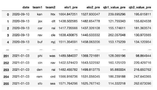
To merge these rankings onto our aggregated dataset, and create the differential rating features:
def merge_rankings(agg_games_df,elo_df):
    agg_games_df = pd.merge(agg_games_df, elo_df, how = 'inner', left_on = ['home_abbr', 'away_abbr'], right_on = ['team1', 'team2']).drop(columns = ['date','team1', 'team2'])
    agg_games_df['elo_dif'] = agg_games_df['elo2_pre'] - agg_games_df['elo1_pre']
    agg_games_df['qb_dif'] = agg_games_df['qb2_value_pre'] - agg_games_df['qb1_value_pre']
    agg_games_df = agg_games_df.drop(columns = ['elo1_pre', 'elo2_pre', 'qb1_value_pre', 'qb2_value_pre'])
    return agg_games_df
Now we can consolidate all the separate functions into a single function. We also want to prepare the dataset for training by splitting the games that have already been played from those that have not (and of course, we also want to create a prediction).
def prep_test_train(current_week,weeks,year):
    current_week = current_week + 1
    schedule_df  = get_schedule(year)
    weeks_games_df = game_data_up_to_week(weeks,year)
    agg_games_df = agg_weekly_data(schedule_df,weeks_games_df,current_week,weeks)
    elo_df = get_elo()
    agg_games_df = merge_rankings(agg_games_df, elo_df)
    train_df = agg_games_df[agg_games_df.result.notna()]
    current_week = current_week - 1
    test_df = agg_games_df[agg_games_df.week == current_week]
    return test_df, train_df
The current_week argument of the function is the week that we want to predict.
Finally, to run everything for week 9 of the NFL schedule:
current_week = 9
weeks = list(range(1,current_week + 1))
year = 2020
pred_games_df, comp_games_df = prep_test_train(current_week,weeks,year)
The pred_games_df gives us the following results:
And the comp_games_df gives us the following:
6 – Training a Model to Predict NFL Games
Now that we have divided the dataset into games we want to predict and games that have already been played, we can train our model and use it to predict the game outcomes. We start with a simple logistic regression model to provide a baseline performance.
But before we get to training the model, we’ll want a convenient way to display the predicted probabilities. The following display function takes the predicted probabilities as an input and prints out a prediction:
def display(y_pred,X_test):
    for g in range(len(y_pred)):
        win_prob = round(y_pred[g],2)
        away_team = X_test.reset_index().drop(columns = 'index').loc[g,'away_name']
        home_team = X_test.reset_index().drop(columns = 'index').loc[g,'home_name']
        print(f'The {away_team} have a probability of {win_prob} of beating the {home_team}.')
Now we can split the dataframe containing our completed games into a test and training set, and drop the columns that are not relevant to the model.
msk = np.random.rand(len(comp_games_df)) < 0.8
train_df = comp_games_df[msk]
test_df = comp_games_df[~msk]
X_train = train_df.drop(columns = ['away_name', 'away_abbr', 'home_name', 'home_abbr', 'week','result'])
y_train = train_df[['result']]
X_test = test_df.drop(columns = ['away_name', 'away_abbr', 'home_name', 'home_abbr', 'week','result'])
y_test = test_df[['result']]
To train the model, run the following:
from sklearn.linear_model import LogisticRegression
clf = LogisticRegression(penalty='l1', dual=False, tol=0.001, C=1.0, fit_intercept=True,
                   intercept_scaling=1, class_weight='balanced', random_state=None,
                   solver='liblinear', max_iter=1000, multi_class='ovr', verbose=0)
 clf.fit(X_train, np.ravel(y_train.values))
y_pred = clf.predict_proba(X_test)
y_pred = y_pred[:,1]
display(y_pred,test_df)
The output should look similar to the following:
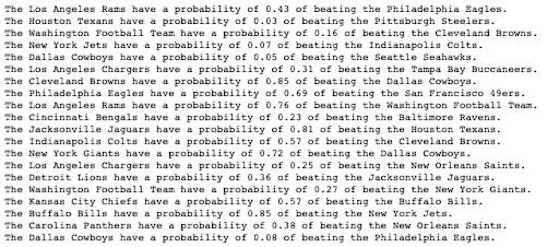
Since these games have already been played, we can compare the predictions to the actual game results (assuming a cutoff probability of 50%):
from sklearn.metrics import accuracy_score
accuracy_score(y_test,np.round(y_pred))
0.75
Not bad: a simple logistic regression picks 75% of the games correctly. So now that we have a baseline, we can implement a more sophisticated model. We could try using gradient boosting within the logistic regression model to boost model performance. But extreme gradient boosting is an algorithm that involves building multiple weak predictive models and iteratively minimizing a cost function that results in a single strong predictive model.
To try these out, we can use the xgboost package. The package allows us to predict an outcome of 0 or 1 directly, instead of just predicting the probabilities and then thresholding. To implement this:
import xgboost as xgb
dtest = xgb.DMatrix(X_test, y_test, feature_names=X_test.columns)
dtrain = xgb.DMatrix(X_train, y_train,feature_names=X_train.columns)
param = {'verbosity':1,
         'objective':'binary:hinge',
         'feature_selector': 'shuffle',
         'booster':'gblinear',
         'eval_metric' :'error',
         'learning_rate': 0.05}
 evallist = [(dtrain, 'train'), (dtest, 'test')]
And to run:
num_round = 1000
bst = xgb.train(param, dtrain, num_round, evallist)
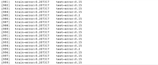
The model performs a bit better than logistic regression alone, obtaining a final accuracy score of 85%:
7 – Predicting NFL Game Outcomes
Finally, we can use this model to make predictions on the games occurring from week 9. At the time of writing, week 9 games have not yet occurred, so it will be interesting to see how the model performs!
To predict the probabilities using our logistic regression model:
X_test = pred_games_df.drop(columns = ['away_name', 'away_abbr', 'home_name', 'home_abbr', 'week','result'])
y_pred = clf.predict_proba(X_test)
y_pred = y_pred[:,1]
display(y_pred,pred_games_df)

Editor’s Note: week 9 predictions were 71% correct
Using Python to predict NFL Winners – Summary
In this tutorial, we used Python to build a model to predict the NFL game outcomes for the remaining games of the season using in-game metrics and external ratings.
While I presented the entire process in a linear manner, the reality of creating a model like this is quite the opposite. A model should be developed recursively, such that more data can be added, additional features included, and different training parameters varied. I encourage all readers to try to improve their own models with additional model tuning and feature engineering. Good luck!
- My code can be found on my GitLab repository here.
- Sign up for a free ActiveState Platform account so you can download the NFL Game Prediction Python environment for Windows or Linux and start predicting NFL games today!


