How to Slice a DataFrame in Pandas

Pandas DataFrame syntax includes “loc” and “iloc” functions, eg.,  data_frame.loc[ ] and data_frame.iloc[ ]. Both functions are used to access rows and/or columns, where “loc” is for access by labels and “iloc” is for access by position, i.e. numerical indices. 

Slicing a DataFrame in Pandas includes the following steps:

1. 1. Ensure Python is installed (or install ActivePython)
   2. Import a dataset
   3. Create a DataFrame
   4. Slice the DataFrame

Note: Video demonstration can be watched here

>> import pandas as pd
>> pd.__version__

>> 0.22.0

data_frame = pd.read_csv("name_of_the_file.csv")

Here we use the “read_csv” parameter. Other types of data would use their respective read function parameters. 

#3 Creating a DataFrame

Besides creating a DataFrame by reading a file, you can also create one via a Pandas Series. Series are one dimensional labeled Pandas arrays that can contain any kind of data, even NaNs (Not A Number), which are used to specify missing data. Let’s create a small DataFrame, consisting of the grades of a high schooler:

classes = pd.Series(["Mathematics","Chemistry","Physics","History","Geography","German"])
grades  = pd.Series([90,54,77,22,25])
pd.DataFrame({"Classes": classes, "Grades": grades})

The result should look like:

Apart from the fact that our example student has pretty bad grades for History and Geography classes, we can see that Pandas has automatically filled in the missing grade data for the German course with “NaN”.

#4 Slicing a DataFrame

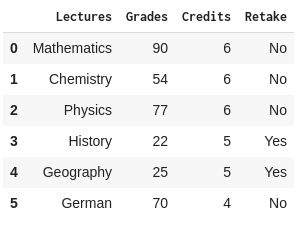
Sometimes generating a simple Series doesn’t accomplish our goals. For more complex operations, Pandas provides DataFrame Slicing using “loc” and “iloc” functions. For example, let’s say Benjamin’s parents wanted to learn more about their son’s performance at the school. They want to see their son’s lectures, grades for these lectures, # of credits earned, and finally if their son will need to take a retake exam. We can simply slice the DataFrame created with the grades.csv file, and extract the necessary information we need. For example:

Grades = 
Report_Card.loc[(Report_Card["Name"] == "Benjamin Duran"),  
               ["Lectures","Grades","Credits","Retake"]]

This might look complicated at first glance but it is rather simple. In this case, we are using the function loc[a,b] in exactly the same manner in which we would normally slice a multidimensional Python array. 

For the a value, we are comparing the contents of the Name column of Report_Card with Benjamin Duran which returns us a Series object of Boolean values. We are able to use a Series with Boolean values to index a DataFrame, where indices having value “True” will be picked and “False” will be ignored. 

For the b value, we accept only the column names listed. Thus we get the following DataFrame:

We can also slice the DataFrame created with the grades.csv file using the iloc[a,b] function, which only accepts integers for the a and b values. In this case, we can examine Sofia’s grades by running:

Sofia_Grades = Report_Card.iloc[6:12,2:]
or else:
Sofia_Grades = Report_Card.iloc[[6,7,8,9,10,11],[2,3,4,5]]
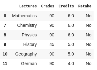
Both of the above code snippets result in the following DataFrame:

In the first line of code, we’re using standard Python slicing syntax: iloc[a,b] where a, in this case, is 6:12 which indicates a range of rows from 6 to 11. When specifying a range with iloc, you always specify from the first row or column required (6) to the last row or column required+1 (12). As you can see in the original import of grades.csv, all the rows are numbered from 0 to 17, with rows 6 through 11 providing Sofia’s grades. This is the result we see in the DataFrame. 

As for the b argument, instead of specifying the names of each of the columns we want as we did with loc, this time we are using their numerical positions. Hence we specify (2:), which indicates that we want all the columns starting from position 2 (ie., Lectures, where column 0 is Name, and column 1 is Class). As shown in the output DataFrame, we have the Lectures, Grades, Credits and Retake columns which are located in the 2nd, 3rd, 4th and 5th columns.

Finally iloc[a,b] can also accept integer arrays as a and b, which is exactly why our second iloc example:

Sofia_Grades = Report_Card.iloc[[6,7,8,9,10,11],[2,3,4,5]]

Produces the same DataFrame as the first example:

Sofia_Grades = Report_Card.iloc[6:12,2:]

This method can be useful for when creating arrays of indices via functions or receiving them as arguments.

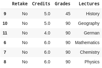
NOTE: It is important to note that the order of indices changes the order of rows and columns in the final DataFrame. If we run the following code:

Sofia_Grades = Report_Card.iloc[[9,10,11,6,7,8],[5,4,3,2]]

The result is the following DataFrame, which shows row indices following the numbers in the indice arrays we provided:

Next steps

Now that you know how to slice a DataFrame in Pandas library, let’s move on to other things you can do with Pandas:

• How to access a row in a DataFrame
• How to group data in Python using Pandas
• View all our articles for the Pandas library
• Read other ‘How-to’ tutorials for Python Packages

Python For Data Science

Pre-bundled with the most important packages Data Scientists need, ActivePython is pre-compiled so you and your team don’t have to waste time configuring the open source distribution. You can focus on what’s important–spending more time building algorithms and predictive models against your big data sources, and less time on system configuration.

Some Popular Python Packages for Data Science/Big Data/Machine LearningYou Get Pre-compiled – with ActivePython

With deep roots in open source, and as a founding member of the Python Foundation, ActiveState actively contributes to the Python community. We offer the convenience, security and support that your enterprise needs while being compatible with the open source distribution of Python.

Download ActiveState Python to get started or contact us to learn more about using ActiveState Python in your organization.

You can also start by trying our mini ML runtime for Linux or Windows that includes most of the popular packages for Machine Learning and Data Science, pre-compiled and ready to for use in projects ranging from recommendation engines to dashboards.