A tragedy like the sinking of the RMS Titanic in 1912, four days into the maiden voyage of the world’s largest ship, can be analyzed from many angles: the historical significance, the geopolitical consequences, or, for the purposes of the Kaggle competition, it can be used as a scenario that can help explain the power of Machine Learning (ML).
The long-running Titanic competition on Kaggle asks you to predict which passengers survived the sinking of the Titanic. Because there weren’t enough lifeboats for everyone, 1502 out of 2224 people on board died, but whether you survived or died was not random. The challenge, then, is to build a predictive model based on the data provided by Kaggle to answer the question: “what kinds of traits characterized survivors?”
This blog post takes the form of a machine learning and Python tutorial in which we’ll examine three different models to determine who survived:
- A simple baseline model
- A basic tree model
- An AutoML-driven (Automatic Machine Learning) model
Our approach to this machine learning implementation will use the following steps:
- Perform an exploratory data analysis to see which of the variables we might want to include in our model
- Examine the baseline model, which is based on a single variable (sex) and yet provides a survivability of 77%. Any model we generate must yield a probability of surviving greater than 0.77.
- Create a decision tree model to see whether we can use multiple variables to yield a higher probability of survival.
- Create a model using AutoML tools.
- Finally, we’ll compare the scores from each method, and analyze the efficacy of each one.
Before you start: Install Our Titanic Competition Ready-To-Use Python Environment
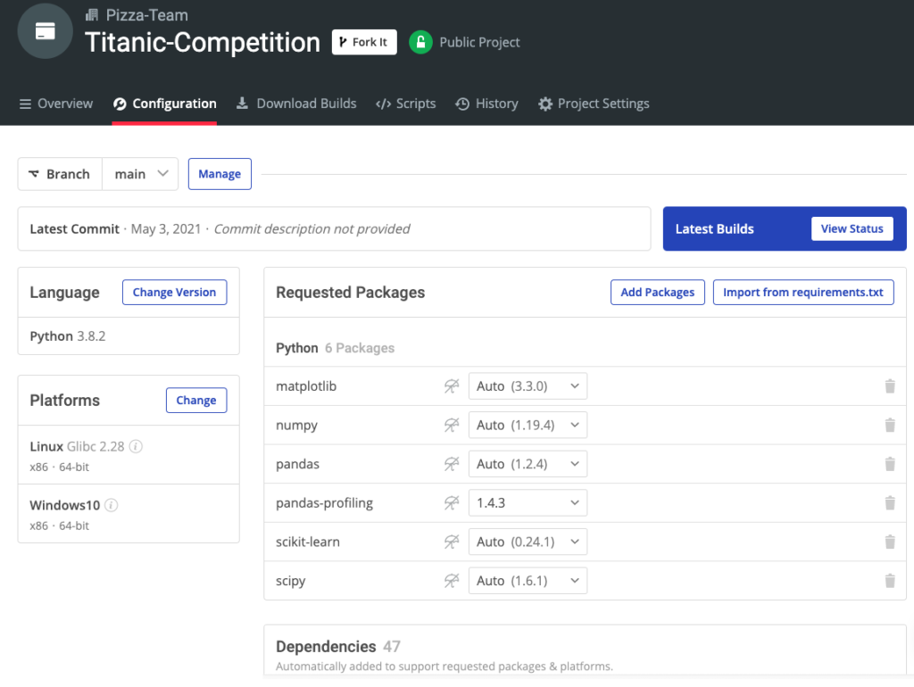
The easiest way to get started creating an entry for Kaggle’s Titanic survivor competition is to install our Titanic Competition Python environment for Windows or Linux, which contains a version of Python and all of the packages you need.
In order to download the ready-to-use Titanic Competition Python environment, you will need to create an ActiveState Platform account. Just use your GitHub credentials or your email address to register. Signing up is easy and it unlocks the ActiveState Platform’s many benefits for you!
Or you could also use our State tool to install this runtime environment.
For Windows users, run the following at a CMD prompt to automatically download and install our CLI, the State Tool along with the Titanic Competition runtime into a virtual environment:
powershell -Command "& $([scriptblock]::Create((New-Object Net.WebClient).DownloadString('https://platform.www.activestate.com/dl/cli/install.ps1'))) -activate-default Pizza-Team/Titanic-Competition"
For Linux users, run the following to automatically download and install our CLI, the State Tool along with the Titanic Competition runtime into a virtual environment:
sh <(curl -q https://platform.www.activestate.com/dl/cli/install.sh) --activate-default Pizza-Team/Titanic-Competition
1–How to Perform an Exploratory Data Analysis
The Titanic dataset provided by Kaggle is split into train and test files. The training file contains a variable called Survived (representing the number of survivors), which is our target. After downloading the dataset, you can perform an automatic Exploratory Data Analysis (EDA) to get a taste of the available variables. We’re going to rely on the pandas-profiling library, as shown below:
import pandas as pd
from pandas_profiling import ProfileReport
df = pd.read_csv('./data/train.csv')
eda_report = ProfileReport(df)
eda_report
The report gives a general overview of the variables, including:
- Number of variables
- Missing values
- Cardinality
- Duplicate rows
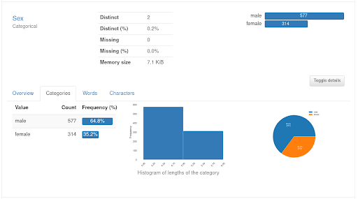
For each numerical variable, you will also get a histogram showing its value and how it correlates with other variables. The details given for the categorical values include the frequency of each category, as in the description of the Sex variable below:
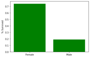
Now that we know which variables are available, we can explore the data in detail in order to find patterns that will help us define a useful model. Let’s start with plotting the relationship between the Sex and Survived variables:
fig, ax = plt.subplots(figsize=(12,8))
gender_count = df['Sex'].value_counts(sort=False)
s_count = df.loc[df['Survived'] == 1, ['Sex']].value_counts(sort=False)
ax.bar('Female', s_count['female']/gender_count['female'], color='green')
ax.bar('Male', s_count['male']/gender_count['male'], color='green')
ax.set_ylabel('% Survived')
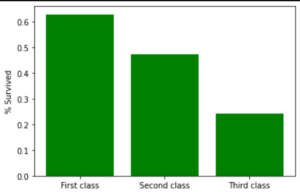
As you can see, more than 70% of female passengers survived, whereas less than 20% of their male counterparts made it out alive. We can examine the ticket class (Pclass) versus the Survived variable in the same way:
fig, ax = plt.subplots(figsize=(6,4))
pclass_count = df['Pclass'].value_counts(sort=False)
s_count = df.loc[df['Survived'] == 1, ['Pclass']].value_counts(sort=False)
ax.bar('First class', s_count.iloc[0]/pclass_count.iloc[0], color='green')
ax.bar('Second class', s_count.iloc[1]/pclass_count.iloc[1], color='green')
ax.bar('Third class', s_count.iloc[2]/pclass_count.iloc[2], color='green')
ax.set_ylabel('% Survived')
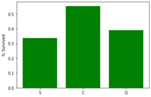
The difference between the three classes is evident, as almost 60% of passengers with first-class tickets survived. This could give us insight into the evacuation orders, or even tell us how the lifeboats were filled (with preference being given to first-class passengers). We can even check the relationship between the port (S=Southampton, C=Cherbourg, Q=Queenstown) where the passengers embarked and their survival:
fig, ax = plt.subplots(figsize=(6,4))
embarked_count = df['Embarked'].value_counts(sort=False)
s_count = df.loc[df['Survived'] == 1, ['Embarked']].value_counts(sort=False)
ns_count = df.loc[df['Survived'] == 0, ['Embarked']].value_counts(sort=False)
ax.bar('S', s_count['S']/embarked_count['S'], color='green')
ax.bar('C', s_count['C']/embarked_count['C'], color='green')
ax.bar('Q', s_count['Q']/embarked_count['Q'], color='green')
ax.set_ylabel('% Survived')
Given this set of variables, we can come up with numerous theories as to which of them might be more likely associated with survivors. For example, women with first-class tickets who embarked in Cherbourg seem to have a far greater chance of surviving than a man with a third-class ticket who embarked at Southampton. Now, let’s move on to our models.
2–Examining the Baseline Model
As Kaggle’s Titanic tutorial explains, the data for the competition includes a sample submission file that assumes all female passengers survived. This is known as a baseline model, which means that it’s the simplest model that can be built from the data without requiring any deeper analysis besides a small verification. In this example, the percentage of female versus male survivors supports the hypothesis that gender is a good predictor of survival.
The score for this baseline model is over 0.7, and any new model that we submit should have a better score.
3–How to Create a Decision Tree Model
The first step in building a good model is to make sure we start with clean, workable data, so we’ll need to work on the dataset a bit. Since Sex is important but only has two possible variables, we can transform M and F to numerical values using the scikit-learn preprocessing class LabelEncoder, which assigns a unique integer to each column’s label in the DataFrame:
df['Sex'] = preprocessing.LabelEncoder().fit_transform(df['Sex'])
df['Embarked'] = preprocessing.LabelEncoder().fit_transform(df['Embarked'])
df[['Sex','Embarked']].info()
<class 'pandas.core.frame.DataFrame'>
RangeIndex: 891 entries, 0 to 890
Data columns (total 2 columns):
#   Column    Non-Null Count  Dtype
---  ------    --------------  -----
0   Sex       891 non-null    int64
1   Embarked  891 non-null    int64
dtypes: int64(2)
memory usage: 14.0 KB
Remember our theory that a first-class woman from Cherbourg had a much better chance of surviving than a third-class man from Southampton? Well, it can be modeled as a decision tree, and you can train a class to make predictions based on this kind of analysis using scikit-learn. The idea here is that the algorithm can infer some rules based on the features passed as training data, and then apply those rules to make predictions when given new data:
X = df[['Sex','Pclass','Embarked']]
y = df['Survived']
clf = DecisionTreeClassifier(random_state=42)
scores = cross_val_score(clf, X, y, cv=5)
print("Mean accuracy for 5 folds", scores)
----------------------------------------------------------------------
Mean accuracy for 5 folds [0.80446927 0.82022472 0.83146067 0.78651685 0.81460674]
Here, we defined three features from the DataFrame to be used in training the DecisionTreeClassifier instance:
- Sex
- Pclass
- Embarked
The Cross_val_score performs five iterations in which it selects some data for training and some for testing. It then fits the DecisionTreeClassifier instance and evaluates the results using the default metric of the algorithm, which was the accuracy (the number of good results / total tests performed), in this example. The results were better than the baseline model in all cases, so now we can train a model and predict the results with the test dataset:
#fit the model with all train data
clf.fit(X,y)
#Load and transform the test data
df_test = pd.read_csv('./data/test.csv')
df_test['Sex'] = preprocessing.LabelEncoder().fit_transform(df_test['Sex'])
df_test['Embarked'] = preprocessing.LabelEncoder().fit_transform(df_test['Embarked'])
#Predict over the test dataframe
predictions = clf.predict(df_test[['Sex','Pclass','Embarked']])
#prepares a dataframe to be submitted
df_submission = pd.DataFrame({'PassengerId':df_test['PassengerId'], 'Survived':predictions})
#data types must be exactly the same as the training data
df_submission.Survived = df_submission.Survived.astype(int)
#only saves the two columns into the submission csv file
df_submission.to_csv( './results/baseline_submission.csv',index=False )
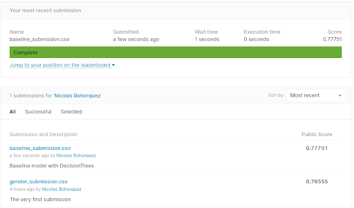
As you can see, our code loads the test dataset and performs the same transformations that we used in the training data. Then it makes predictions and saves the results in a CSV file, keeping track of the type of data in the prediction. Kaggle evaluates the incorrect predictions with a different type of data than the one used in training. The results are slightly worse than they were with the single variable:
4–How to use AutoML Tools to Create a Model
We really need a deeper analysis to extract more information from the data. We also need to play with the algorithms and the hyperparameters to properly tune the desired method of classification. But that’s going to be a lot of work, so instead let’s give the automated tooling a chance to see how much it can improve our baseline model.
The team behind the MLBox project assembled an analysis for the Titanic dataset that includes full preprocessing, algorithm selection, hyperparameter tuning, training, predicting, and even packaging the results for submission:
#1. load and preprocess data
paths = ["./data/train.csv","./data/test.csv"]
target_name = "Survived"
rd = Reader(sep = ",")
df_mlbox = rd.train_test_split(paths, target_name)
#2. removes non-stable features
dft = Drift_thresholder()
df = dft.fit_transform(df_mlbox)
#3. optimize defining a search space for each aspect of the algorithms
opt = Optimiser(scoring = "accuracy", n_folds = 5)
space = {
	       'est__n_estimators':{"search":"choice","space":[150]},
       'est__colsample_bytree':{"search":"uniform","space":[0.8,0.95]},
       'est__subsample':{"search":"uniform","space":[0.8,0.95]},
       'est__max_depth':{"search":"choice","space":[5,6,7,8,9]},
       'est__learning_rate':{"search":"choice","space":[0.07]}
       }
params = opt.optimise(space, df,15)
#4. predict using the previously optimized params
prd = Predictor()
prd.fit_predict(params, df)
#5. packaging to submit
submit = pd.read_csv("./results/baseline_submission.csv",sep=',')
preds = pd.read_csv("./save/"+target_name+"_predictions.csv")
submit[target_name] =  preds[target_name+"_predicted"].values
submit.to_csv("./results/mlbox.csv", index=False)
In the above code:
- Step 1 simply uses a reader to load the training and test datasets.
- Step 2 is the most complicated, because it deals with the selection process that not only drops useless variables, but also takes care of the drifting variables. (A drifting variable changes its statistical properties from the training dataset to the test dataset. For more information, check out this link).
- Step 3 optimizes the hyperparameters by setting a search space and fitting the selected algorithm with the training data.
- Step 4 performs the predictions and saves them in an mlbox.csv file.
- Step 5 prepares the predictions for submission to Kaggle.
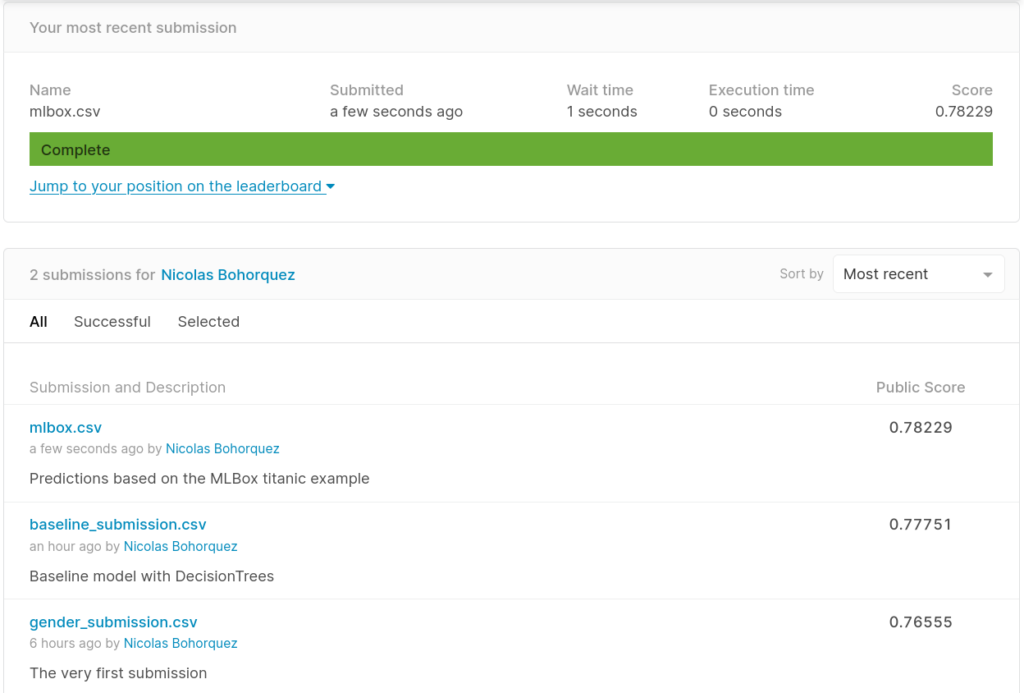
As you can see, the predictions made by the AutoML model were slightly better than the baseline model. The lesson is clear: the automatic model was better parametrized, but it still lacks the feature engineering that a human could contribute.
Conclusion: Kaggle’s Titanic Competition with ActivePython – a faster simpler way to results
Kaggle’s Titanic competition has been around for years and currently has more than 160,000 entries! It’s unlikely that our quick and dirty approach is going to provide us with winning results, but it will get you much more familiar with the Kaggle platform, which is one of the best for learning Machine Learning.
That said, there’s still a lot more you can do with the data provided by the Titanic dataset. Our scores from the baseline model, the simple decision tree model, and the AutoML model are okay, but they could be greatly improved by working with the features, algorithms, and hyperparameters available in the Python libraries for machine learning.
The simplest way to get started is to:
- Review the code for this project in my repo on GitHub.
- Download the Titanic Competition environment for Windows and Linux, which includes a version of Python and all the packages you need to create your own entry.
With the ActiveState Platform, you can create your Python environment in minutes, just like the one we built for this project. Try it out for yourself or learn more about how it helps Python developers be more productive.
Related Reads
The Top 10 AutoML Python packages to automate your machine learning tasks


