
Using ActivePython ensures you get the most out of TensorFlow and your hardware. They do all the optimization for you, and it is simple to install and use. When scaling models to larger datasets, using ActivePython is a guaranteed way to ensure your TensorFlow models are optimized to the fullest.
Download our ActivePython for Anaconda distribution for Windows or Linux. It features most of the packages Anaconda users are used to, along with our version of TensorFlow so you can test it out for yourself.
TensorFlow has become one of the most popular machine learning software packages among data scientists. It was originally developed for internal use at Google before being released under an open source license in 2015. The library is based on the use of computational graphs, where the nodes of the graph are operations (i.e. addition, subtraction, etc.) and the edges of the graph are tensors. A tensor is just another name for a multidimensional matrix. For example, a computational graph for the addition of two tensors looks like this:
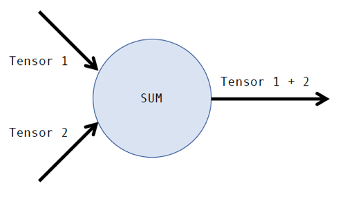
Of course, the addition of two tensors is a relatively simple operation to perform computationally. Many more sophisticated operations lie within machine learning algorithms. The time it takes to train a machine-learning model depends on a variety of factors, such as the complexity of the operations, the size of the tensors, and the underlying hardware being utilized. Whether or not a data scientist is getting the most out of their TensorFlow model depends heavily on optimizing these factors.
Both the operators and entire graphs can be optimized. Operator-level optimizations can be made to ensure that basic math operations are executed in the most efficient way for the specific processors being used. Additionally, further graph optimizations can be done:
- Efficient data layout to avoid any unnecessary data shuffling while training
- Proper memory allocation so no space is wasted
- Load balancing to exploit parallelism within and between operations
- Node merging to identify if any operations that are commonly repeated can be merged
Ensuring model optimization can save time and money, especially when being scaled to large datasets. Fortunately, ActiveState provides a ready to install, pre-built distribution of Python called ActivePython. When considering the aforementioned optimization strategies, ActivePython is designed to extract the most out of a TensorFlow model. In this article, I’ll build a TensorFlow model and compare the performance with and without ActivePython.
Building the Model
I’ll use the wine dataset from the UCI Machine Learning Repository. The dataset contains 178 observations of wine grown in the same region in Italy. Each observation is from one of three cultivars (the ‘Class’ feature), with 13 constituent features that are the result of a chemical analysis. We will build a model using TensorFlow that predicts the correct cultivar of each wine. You can find the code in the Python file here.
First, we’ll import the data and load the relevant libraries:
import pandas as pd
import numpy as np
import tensorflow as tf
wine_names = ['Class', 'Alcohol', 'Malic acid', 'Ash', 'Alcalinity of ash', 'Magnesium', 'Total phenols', 'Flavanoids', 'Nonflavanoid phenols', 'Proanthocyanins', 'Color intensity', 'Hue', 'OD280/OD315', 'Proline']
wine_data = pd.read_csv('wine.data', names = wine_names)
wine_df = pd.DataFrame(wine_data)
wine_df_x = wine_df.loc[:,'Alcohol':'Proline']
wine_df_y = wine_df.loc[:,'Class']
We’ll split the dataset into a test set and a training set, using the former to test the model once it has been trained with the latter. For TensorFlow, we need to convert the data to a format that it can understand – a tensor:
from sklearn.model_selection import train_test_split
def convertClass(val):
    if val == 1:
        return [1, 0, 0]
    elif val == 2:
        return [0, 1, 0]
    else:
        return [0, 0, 1]
		Y = wine_df.loc[:,'Class'].values
Y = np.array([convertClass(i) for i in Y])
X = wine_df.loc[:,'Alcohol':'Proline'].values
train_x, test_x, train_y, test_y = train_test_split(X,Y , test_size=0.3, random_state=0)
train_x = train_x.transpose()
train_y = train_y.transpose()
test_x = test_x.transpose()
test_y = test_y.transpose()
We’ll also need to define a couple of functions to provide the basis for our neural net. I won’t go into the details of how neural nets are constructed and the mathematics behind them, but there are plenty of great resources available. I recommend this online textbook.
def init_parameters(num_input_features):
    num_hidden_layer =  50
    num_hidden_layer_2 = 13
    num_output_layer_1 = 3
	    tf.set_random_seed(1)
    W1 = tf.get_variable("W1", [num_hidden_layer, num_input_features], initializer = tf.contrib.layers.xavier_initializer(seed=1))
    b1 = tf.get_variable("b1", [num_hidden_layer, 1], initializer = tf.zeros_initializer())
    W2 = tf.get_variable("W2", [num_hidden_layer_2, num_hidden_layer], initializer = tf.contrib.layers.xavier_initializer(seed=1))
    b2 = tf.get_variable("b2", [num_hidden_layer_2, 1], initializer = tf.zeros_initializer())
    W3 = tf.get_variable("W3", [num_output_layer_1, num_hidden_layer_2], initializer = tf.contrib.layers.xavier_initializer(seed=1))
    b3 = tf.get_variable("b3", [num_output_layer_1, 1], initializer = tf.zeros_initializer())
	    parameters = {"W1": W1,
                  "b1": b1,
                  "W2": W2,
                  "b2": b2,
                  "W3": W3,
                  "b3": b3}
				      return parameters
	def for_prop(X, parameters):
    W1 = parameters['W1']
    b1 = parameters['b1']
    W2 = parameters['W2']
    b2 = parameters['b2']
    W3 = parameters['W3']
    b3 = parameters['b3']
	    Z1 = tf.add(tf.matmul(W1, X), b1)
    A1 = tf.nn.relu(Z1)
    Z2 = tf.add(tf.matmul(W2, A1), b2)
    A2 = tf.nn.relu(Z2)
    Z3 = tf.add(tf.matmul(W3, A2), b3)
    return Z3
	def c(Z3, Y):
    logits = tf.transpose(Z3)
    labels = tf.transpose(Y)
    cost = tf.reduce_mean(tf.nn.softmax_cross_entropy_with_logits_v2(logits=logits, labels=labels))
    return cost
 def rand_batches(X, Y, batch_size = 128, seed = 0):
    m = X.shape[1]
    batches = []
    np.random.seed(seed)
	    # Step 1: Shuffle (X, Y)
    permutation = list(np.random.permutation(m))
    shuffled_X = X[:, permutation]
    shuffled_Y = Y[:, permutation].reshape((Y.shape[0],m))
	    # Step 2: Partition (shuffled_X, shuffled_Y). Minus the end case.
    num_batches = math.floor(m/batch_size)
    for k in range(0, num_batches):
        batch_X = shuffled_X[:, k * batch_size : k * batch_size + batch_size]
        batch_Y = shuffled_Y[:, k * batch_size : k * batch_size + batch_size]
        batch = (batch_X, batch_Y)
        batches.append(batch)
		    # Handling the end case (last mini-batch < mini_batch_size)
     if m % batch_size != 0:
        batch_X = shuffled_X[:, num_batches * batch_size : m]
        batch_Y = shuffled_Y[:, num_batches * batch_size : m]
        batch = (batch_X, batch_Y)
        batches.append(batch)
		     return batches
Finally, we’ll define a final function that pieces together all the previously defined functions. After initializing the tensors and parameters, we’ll set up forward propagation and the cost function. Then we’ll train our model on the defined cost function for a set number of epochs, and run the test set through the model:
from tensorflow.python.framework import ops
import math
import time
def nn(train_x, train_y, test_x, test_y, learning_rate ,num_epochs, batch_size, print_cost = True):
        ops.reset_default_graph()
        tf.set_random_seed(1)
		        (n_x, m) = train_x.shape
        n_y = train_y.shape[0]
		        #initialize
        costs = []
        X = tf.placeholder(tf.float32, [n_x, None], name="X")
        Y = tf.placeholder(tf.float32, [n_y, None], name="Y")
        parameters = init_parameters(13)
		        # Forward propagation: Build the forward propagation in the tensorflow graph
        Z3 = for_prop(X, parameters)
        cost = c(Z3, Y)
        optimizer = tf.train.AdamOptimizer(learning_rate=learning_rate).minimize(cost)
        init = tf.global_variables_initializer()
		        with tf.Session() as sess:
            sess.run(init)
			            #training loop
            for epoch in range(num_epochs):
			                epoch_cost = 0.
                start = time.time()
                num_batches = int(m / batch_size)
                batches = rand_batches(train_x, train_y, batch_size, 13)
				                for batch in batches:
                    (batch_X, batch_Y) = batch
                    _ , batch_cost = sess.run([optimizer, cost], feed_dict={X: batch_X, Y: batch_Y})
                    epoch_cost += batch_cost / num_batches
					                # Print the cost every epoch
                if print_cost == True and epoch % 100 == 0:
                    print ("Epoch %i cost: %f" % (epoch, epoch_cost))
                    print ('Time taken for this epoch {} sec\n'.format(time.time() - start))
                if print_cost == True and epoch % 5 == 0:
                    costs.append(epoch_cost)
					            # lets save the parameters in a variable
            parameters = sess.run(parameters)
            print("Parameters trained...")
			            # Calculate the correct predictions
            correct_prediction = tf.equal(tf.argmax(Z3), tf.argmax(Y))
			            # Calculate accuracy on the test set
            accuracy = tf.reduce_mean(tf.cast(correct_prediction, "float"))
			            print("Train Accuracy:", accuracy.eval({X: train_x, Y: train_y}))
            print("Test Accuracy:", accuracy.eval({X: test_x, Y: test_y}))
			            return parameters
In the code above, I’ve printed out the cost function and processing time at each 100th epoch. This will allow us to evaluate how well TensorFlow is optimized. Next, I’ll define a variable learning rate, number of epochs, and batch size for model training. Feel free to change these values to see how they affect the outcome:
learning_rate = 0.001 #change this to change learning rate
num_epochs = 1000     #change this to change number of epochs
batch_size = 15       #change this to change batch size
parameters = nn(train_x, train_y, test_x, test_y, learning_rate ,num_epochs, batch_size)
Now that we have our TensorFlow model, we can run it with and without ActivePython and compare the results.
Comparing the Performance
First, I’ll run the model using the standard Python library. To do this, I’ll activate a new conda environment (I prefer to use Anaconda’s Python distribution on my machine) called py365 within Terminal by running:
conda create --name py365 python=3.6.5 --channel conda-forge
conda activate py365
You may need to install a few packages. To do this, run:
conda install pandas
conda install tensorflow
conda install scikit-learn
After installation, you can run our python file (must be within the same directory):
python3.6 TensorFlow_UCIwine.py
If the file runs successfully, you should see an output like this:
Epoch 0 cost: 28.296729
Time taken for this epoch 0.25333499908447266 sec
Epoch 100 cost: 0.355506
Time taken for this epoch 0.009265899658203125 sec
Epoch 200 cost: 0.234137
Time taken for this epoch 0.008865118026733398 sec
Epoch 300 cost: 0.176384
Time taken for this epoch 0.008792877197265625 sec
Epoch 400 cost: 0.143405
Time taken for this epoch 0.008754968643188477 sec
Epoch 500 cost: 0.122086
Time taken for this epoch 0.008751153945922852 sec
Epoch 600 cost: 0.107237
Time taken for this epoch 0.008697748184204102 sec
Epoch 700 cost: 0.094254
Time taken for this epoch 0.008578062057495117 sec
Epoch 800 cost: 0.087498
Time taken for this epoch 0.009491920471191406 sec
Epoch 900 cost: 0.080642
Time taken for this epoch 0.008537054061889648 sec
Parameters trained...
Train Accuracy: 0.9919355
Test Accuracy: 0.9444444
The results obtained are not too bad. Our model correctly predicted 94% of the test set Classes, and the model was trained within a reasonable amount of time.
Next, I’ll run the model using ActivePython. I’m using the free community edition of ActivePython 3.6, which can be found here. Installation instructions can also be found here. To run the model using ActivePython, make sure it’s the default version of Python, and that you have deactivated the conda environment (conda deactivate). You can check this by running (in Terminal):
python3.6
ActivePython should be listed as the default version. To run the model again, use the same command:
python3.6 TensorFlow_UCIwine.py
And a similar output should appear:
Epoch 0 cost: 28.296728
Time taken for this epoch 0.04816007614135742 sec
Epoch 100 cost: 0.355505
Time taken for this epoch 0.004086971282958984 sec
Epoch 200 cost: 0.234135
Time taken for this epoch 0.006526947021484375 sec
Epoch 300 cost: 0.176385
Time taken for this epoch 0.005736351013183594 sec
Epoch 400 cost: 0.143405
Time taken for this epoch 0.0045087337493896484 sec
Epoch 500 cost: 0.122086
Time taken for this epoch 0.004789829254150391 sec
Epoch 600 cost: 0.107235
Time taken for this epoch 0.006066322326660156 sec
Epoch 700 cost: 0.094713
Time taken for this epoch 0.004540205001831055 sec
Epoch 800 cost: 0.087495
Time taken for this epoch 0.004395008087158203 sec
Epoch 900 cost: 0.080680
Time taken for this epoch 0.00403285026550293 sec
Parameters trained...
Train Accuracy: 0.9919355
Test Accuracy: 0.9259259
We obtain a similar testing accuracy of about 93%, but on average, it takes less than half the time for each epoch!
Conclusions
Clearly, using ActivePython ensures you get the most out of TensorFlow and your hardware. They do all the optimization for you, and it is simple to install and use. When scaling models to larger datasets, using ActivePython is a guaranteed way to ensure your TensorFlow models are optimized to the fullest.
- To view all the code and data used in this post, you can refer to my Gitlab repository.
- To run the code, download our ActivePython for Anaconda distribution for Windows or Linux. It features most of the packages Anaconda users are used to, along with our version of TensorFlow so you can test it out for yourself.
Title photo courtesy of maxpixel.net.
Related Blogs:
How to Build a Generative Adversarial Network (GAN) to Identify Deepfakes